| cwave.eu5.org
Also see: http://www.angelfire.com/dragon/letstry cwave04 at yahoo dot com |
 Last updated on Tue May 25 14:31:16 IST 2010. |
|

Factorial design (part 3)
ANOVA
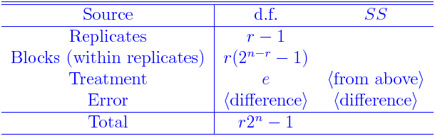
Here we shall consider a (2n ,2k ) experiment in r replicates. Constructing the ANOVA table is not entirely trivial. We split the process in 3 steps:- Constructing Yate's SD table
- Constructing Treatment SS table
- Constructing the ANOVA table
Step 1: Yate's SD table
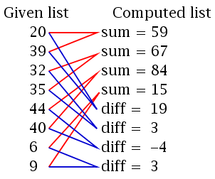
The first step is to compute the SD table. Here SD stands for ``Sum and Difference''. The SD table gives the ''effect totals'' for all the effects (totally confounded, partially confounded, not confounded). Recall that each effect has value either 0 or 1 for each run. The effect total is just the total of all observations for runs with value 1 minus the total for runs with value 0. Yate's SD table is an efficient way to compute these by hand. We shall discuss this table in the next section. Let us denote the effect total for an effect X by CX. For example, we shall have CA, CAB etc. To understand the SD table we have to learn a way to produce a list of number from a given list of numbers. The technique (which we shall call ``SD operation'')works only with lists of even length. It is best explained throgh an example:
 |
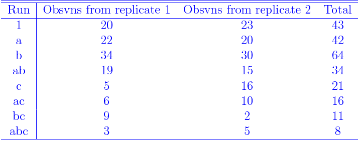
Now we shall apply the SD operation on the last column n times (i.e., 3 times in our case.
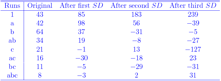
The final columns give the CX's. For example, CA = -39. Notice that there is also a C1 from the first row, though there is not effect called 1. This C1 is nevertheless useful for crosschecking. It will always be the total of all the observations.
Step 2: Treatment SS
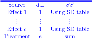
Here The treatment SS is obtained by adding SS due to each effect that is not totally confounded (let the number of such effects be e):Now we shall learn how to find the SS dues to X (which we shall call SSX) from CX. There are two cases:
- If X is not confounded:
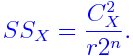
···(notconf) - If X is partially confounded: then the formula must
take into account which replicates confound X and which
don't. Cx is the sum total for all the replicates.
We have to remove the contribution of the replicates where
X is confounded. This is done as
whereCX* = CX - DX,
Here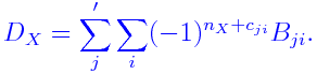
- ∑'j is over replicates j confounding X,
- ∑i is over the 2n-k blocks in the j-th replicate.
- nX= number of factors in X.
- cji = number of factors common between X and any run in the i-th block of the j-th replicate.
- Bji = the total of observations in the i-th block of the j-th replicate.
where r* = number of replicates not confounding X.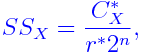
···(parconf)