|
Splitplot Design
The set up
Suppose that we want to conduct an agricultural study with two
treatments:
-
Method of tilling: This has two levels, tractor and
manual.
-
Fertiliser: This has 3 levels, compost, phosphate and
uria.
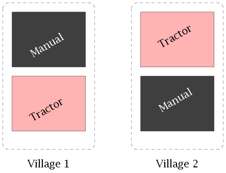
Clearly we need 2×3=6 fields, but we have only 4
large paddy fields for use in the experiment, 2 in one village
and 2 in another.
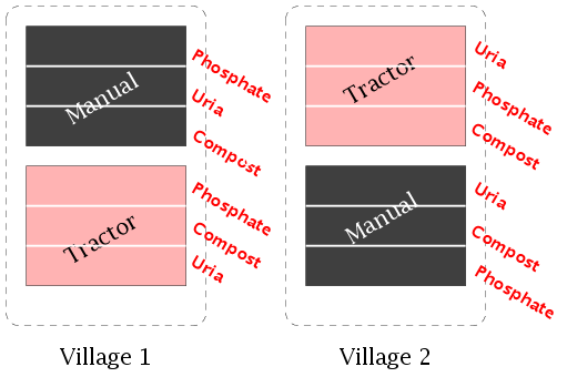
Here we can carry out the experiment as follows.
First we assign methods of tilling to the fields in each village
randomly.
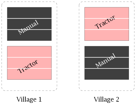
After the fields are tilled they are each split into 3
subfields.
The three fertilisers are assigned randomly to the
subfields in each field.
This design is called a splitplot design.
Let us go through the steps carefully. Instead of fields and
villages we shall use the standard statistical terms. First, a
split plot design is typically used when there are two
treatments (1 and 2) so that treatment 1 is easily applied to
more than one
unit simultaneously. In our example the method of tillage is
treatment 1. It is easier to till a large field at a time using a
single
method, rather than small fields in a peiecemill fashion.
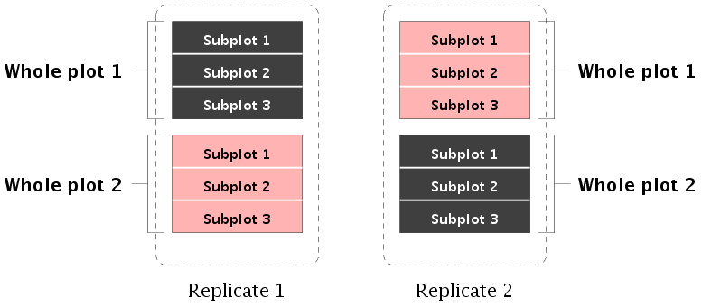
Each field
is called a whole plot, and each subfield is called a
subplot. We had 2 villages with 2 fields each. Each
village is called a replicate. Each replicate consists of
as many whole plots as there are levels of treatment 1. We
randomly assign the levels of treatment 1 to the whole plots in
each replicate.
Then we split each whole plots into as many subplots as there are
levels of treatment 2. These levels are assigned randomly to the
subplots in each whole plot.
We get one value of the response variable (yield of paddy in our
example) per subplot. Thus the subplots are our experimental units.
The model
The model used in a split plot experiment is a mixed effects
model. We shall use the following subscripts:
-
i=1,...,I for replicates,
-
j=1,...,J for levels of treatment 1,
-
k=1,...,K for levels of treatment 2.
The model is
where
-
yijk = yield from (i,j,k)-th subplot
-
μ = (fixed) overall mean effect
-
&alphai = (fixed) extra effect for i-th replicate
-
βj = (fixed) extra effect for j-th level of
treatment 1
-
γk = (fixed) extra effect for k-th level of
treatment 2
-
δjk = (fixed) interaction effect for j-th
level of treatment 1 and k-th level of
treatment 2
-
tij = (random) interaction effect for i-th replicate
and j-th level of treatment 1
-
εijk = random error.
We have the usual assumptions.
First the assumption of the random quantities.
-
εijk's are iid N(0,σe2)
-
tij's are iid N(0,σt2)
- The ε's are independent of the t's.
Then the assumptions of the fixed effect parameters:
-
∑i &alphai = ∑j βj = ∑k γk = 0.
-
∑i δij = ∑j δij = 0.
ANOVA
The ANOVA table for the above model takes the following
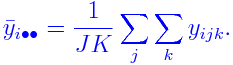
form. Here the bulleted subscripts have been averaged over. For
example,
The ANOVA table is:
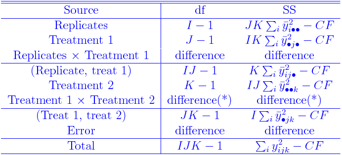
The differences marked with (*) are obtained by subtracting the
Treat 1 and Treat 2 rows from the (Treat 1, treat 2) row.
Also the correction factor (CF) is defined as
Testing
There are various hypotheses of interest. As usual we shall emply
F-tests by taking ratios of appropriate MS
terms. However, we need to be a bit careful here since the
denominator is not always the Error MS! Here is alist of the
different F-ratios.
- To test H0: βj's are all 0 (i.e.,
Treatment 1 has no effect, or both the tilling methods are
equivalent w.r.t. yield) we have to divide the Treat 1 MS
by the Replicate × Treat 1 MS.
- To test H0: γk's are all 0 (i.e.,
Treatment 2 has no effect, or all the fertilisers are
equivalent w.r.t. yield) we have to divide the Treat 2 MS
by the Error MS.
- To test H0: δjk's are all 0 (i.e.,
Treatment 1 has no interaction with treatment 2)
we have to divide the Treat 1 × Treat 2 MS
by the Error MS.
Finding E(MS)
Each of the MS terms is a function of the random data, and
hence are random variables. It is useful to compute their
expectations. The following example illustrates the technique.
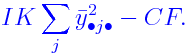
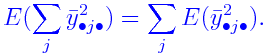
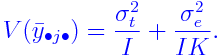
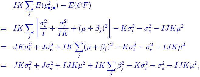
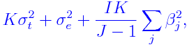
|




 and E(CF)
separately.
and E(CF)
separately.