Set up: We have data X from unknown (joint) distribution
F. We want to compute (some aspect of) the distribution of the random variable
T(F, X) possibly involving both the unknown distribution and the
data.
T is a known function. We shall denote this distribution as
Law(T(F,X); F),
the second occurence of F signifying the fact that X is distributed
as F. It is not difficult to see that any statisitical inference problem
(parametric/nonparametric) may be cast into this form.
Example:
Suppose that X1,...,Xn are iid
with common distribution F. Let θ be mean(F). We want to estimate F by
the median, M, of Xi's. Suppose we are interested in knowing the
MSE of this estimator, ie,
E (M(X)-θ)2
This is a function the distribution of the random variable
T(F,X) = M(X)-θ(F)
The bootstrap idea
Note that X is already given to you, so if you know F then you can
always compute Law(T(F,X); F) in principle, since T is a known
function. If direct computation turns out to be too complicated, we may
approximate Law(T(F,X); F) by simulation from F.
However, this is never
going to happen in practice because if you already know F, why on
earth would you ever think of estimating its mean? So the entire
subject of statistical inference revolves around the issue of computing
Law(T(F,X); F) when F is unknown. Parametric statistical inference
solves this problem by assuming that F is known except for finitely many
unknown constants. Classical non-parametric statistics (i.e., the methods
we have learned so far in this course) looks for distribution-free
techniques, i.e., situations where Law(T(F,X); F) is completely known
even though F is not. The idea is that somehow the two occurences of F in
Law(T(F,X); F) cancel each other out.
Example:
Let X1,...,Xn be iid continuous unknown F with
median θ(F). Define
T(F,X) = sign test statistic based on
(Xi-θ(F))'s
Then
Law(T(F,X); F) = Binomial(n,1/2),
free of F.
This is a smart technique, but the trouble is that there are many
situations where such distribution-free technique is not known to
exist. Even
when one does exist, it often fails to utilise the entire data (e.g.,
it is
based only ranks or signs, and not the actual values.)
Now we are going to learn about a third method called bootstrapping
that lets us approaximate
Law(T(F,X); F)
where F is unknown in even non-distrn-free situations. Thus,
bootstrapping is a method that lets you have the advantage of knowing F,
even when you actually do not know it. Here's the idea:
Try to approximate F by some
distribution F* (may depend on the data X) that
is "close" to F
is completely known
can be easily simulated from.
Use F* as a proxy for F.
Thus, instead of computing Law(T(F,X); F) we actually compute Law(T(F*,X); F*). Note
that Law(T(F*,X); F*) is a known function of X. So at least in
principle we can compute it for any given X. This is called the
ideal bootstrap distribution. In practice, however, even Law(T(F*,X); F*)
may be very complicated. So then we can simulate X* from
F*, and approximate Law(T(F*,X); F*) by a histogram. This called
empirical bootstrap distribution.
Parametric bootstrap
This is a trivial example just to illustrate ideas. Suppose X
consists of X1,...,X200 iid
N(μ,σ2),
μ and σ2 being
unknown.
Estimate μ, σ2 from the data as and
S2. Take F* = N(,S2).
Clearly it is completely known and easy to simulate from.
Exercise:
Compute the idea bootstrap estimate of the bias of for
μ,i.e.,
E(-μ).
Also, compute the ideal bootstrap estimate of the MSE.
Of course, we would never do bootstrap for this problem, because here
we could have done direct computation. It was only for didactic purpose.
The next exercise is slightly more nontrivial.
Exercise:
Suppose that X1,...,X1000 are iid
N(0,σ2). We want to estimate E(X14) by
∑
Xi4/1000.
Compute the ideal bootstrap estimate of its MSE. If that seems too
complicated, then simulate to get emipirical bootstrap estimate.
Nonparametric bootstrap
This is by far the most common form of bootstrap. Many people mean
only this when they talk about bootstrap.
Simplest case
Let us consider the simplest case of nonparametric bootstrap. Here
X consists of X1,...,Xn
iid from some unknown F. We know
nothing about F. One popular choice of F* here is Fn, the
empirical
distribution function, defined as follows.
Let us check if Fn satisfies the three
conditions above.
Close to F ?
The following results are well known about the
proximity of Fn to F.
Exercise:
Prove the following theorem.
Proof:
Shall not prove in this course.
[Q.E.D.]
Completely known ?
Fn is completely known, since it is just a function of the
data.
Easy to simulate ?
Exercise:
Suggest an algortihm to simulate iid from Fn. In particular,
show that if x is a vector of length n storing the original sample then
the Matlab code
bootData = x(unidrnd(n,1,n));
fills up the vector bootData with n iid sample from Fn.
A sample of size n drawn from Fn is called a resample.
In S-plus the function
sample
lets you draw
such a sample (read its help to learn how!)
Exercise:
The file boot.txt
has a sample of size 1000. Draw 100
resamples each of size 1000. Make the histogram of the 100 (5%-)trimmed
means. Actually, the data came from N(0,1) distribution. Generate 100
samples (each of size 1000) from N(0,1), compute (5%-)trimmed means
for each of these samples, and draw the histogram of the 100 trimmed
means. Compare with the bootstrap histogram.
Both S-plus and Matlab have more sophisticated functions to
perform bootstrapping. We shall learn about them in due course.
Exercise:
Suppose that we have some iid data of size n. R(X) is an estimator
for θ, which is some parameter
of interest. Write down the algorithm for computing empirical nonparametric
bootstrap estimates of bias, variance and MSE of R(X).
Exercise:
Estimate mse, bias and variance of the sample median based on the sample
stored in the file boot2.txt.
Working like a pro
Now, bootstrapping is such a popular method, that it is only expected that
S-plus/Matlab will provide special functions to write the above code more
compactly. Indeed, S-plus provides a function called
bootstrap
to implement
the loop in the bootstrap flowchart. If we have a function called, say,
myStatistic(data), that computes T from data, then the code
> bootVal <- bootstrap(data, 1000, myStatistic)
will perform the above loop and store various relevant things in the
variable
bootVal
. Here 1000 is the number of bootstrap
resamples drawn. In particular, bootVal$replicates will
store Ti's. Type
> names(bootVal)
to see what other info
bootVal
stores.
Though the
bootstrap
function is easy to use, it is
important to be able to write your own code for bootstrap. This is because
there are certain scenarios where the standard function cannot be used. We
shall take a look at one such case in a later lecture.
Matlab has a similar function called
bootstrp
(no 'a' !). However, we prefer S-plus for
bootstrapping, because S-plus provides some nice supporting
routines for bootstrap for computing various related quantities.
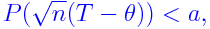
Exercise:
We have some iid data, and some statistic T and a parameter θ.
Suggest how we can use bootstrapping to estimate
for some given number a. [Hint: If the underlying distribution is F, then θ =
θ(F). θ is a known function.]
Exercise:
suppose that we want to estimate standard error of sample mean based on
iid data
X1,...,Xn.
Let R(X;B) be the empirical bootstrap estimator based on B resamples.
Does R(X;B) converge as B goes to infinity?
Exercise:
Draw a resample of size n from
X1,...,Xn,
The Xi's are all distinct.
What is the chance that X1 is not
in the resample? Find the limit as n goes to infinity.
Exercise:
Suggest how you can use bootstrapping to get CI for a parameter.
Trouble with bootstrap
The bootstrap intuition relies on the hope that if F* is close
to F, then Law(T(F*,X); F*) is close to Law(T(F,X); F). Unfortunately, this is not
always true. One such case is given below.
Exercise:
Suppose that we have an iid data from Unif(0,θ). Compute mle
. We want to compare
Law(T(F*,X); F*) with Law(T(F,X); F),
where
T(F,X) = (X)
Suppose that for a particular dataset of size n, the maximum is 1.97.
Compute true P( = 1.97), and also ideal bootstrap estimator of
the same quantity. Take limit of both as n goes to infinity. Do they
match?
What is the implication?
More general set up
So far we have performed bootstrapping only for univariate iid data. It is
possible to do bootstrapping for general data.
Multivariate iid data
It is easy to
generalise to multivariate set up.
Exercise:
Suppose we have paired data
(X1,Y1),...,(Xn,Yn),
such that the n pairs are iid some bivariate F(x,y) having correlation
coefficient θ. We plan to estimate θ by the sample
correlation coefficient . Suggest how you may use boostrapping
to estimate bias, variance, MSE of .
Pricipal Component Analysis (PCA)
Suppose that
X1,...,Xn
are iid k-dimensional random vectors with mean 0 and variance matrix A.
Then for any fixed vector v, the random variable
v'X
has mean 0 and variance σ2(v) = v'Av. Let v be some unit
vector. Then v'X is the projection of X along v.
If σ2(v) is large then we would expect a large scatter of
X along v. Thus, the value of σ2(v) for different unit
vectors v, provide an idea about the structure of the multivariate
distribution of X.
PCA is a systematic approach towards finding the v which maximises
σ2(v). Then it finds w to maximise σ2(w) among all w
orthogonal to v, and so on.
The technique is simple and based on the following theorem.
Proof:
You should know from B-I.
[Q.E.D.]
PCA proceeds just by computing the eigen values of the sample variance
matrix, S, say.
Exercise:
Consider the PCA set up as given above. Let the PCA algorithm produce
v1 as the maximiser of σ2(v). Note that v1
is itself a random vector. We want to estimate its variance
matrix. Suggest how you may use bootstrapping here.
Bootstrap for non-iid data
It is possible to do bootstrap for non-iid data like time series. We shall
consider a regression situation. Suppose that we have two variables X and
Y related by the following formula:
Y = a+b*X + error,
errors are iid with some unknown F.
We take some fixed values
x1,...,xn
for X, and observe Y to get the data
Y1,...,Yn.
Assume that the errors are iid. Let ahat and bhat denote the
(least square or whatever)
estimators of a and b. Here the data Yi's are not iid (they are
indep, but not identically distributed.) So here we perform bootstrap as
follows.
We first compute the residuals as
Ri = Yi - ahat - bhat*xi,
Then we approximate F by the empirical distribution, Fn, of
these. Finally we
approximate the distribution of Yi by that of
ahat + bhat*xi + error*,
where error* ~ Fn.
This is called bootstrapping the residuals.
Exercise:
As you might have guessed from the above description, computing the ideal
boostrap distribution is very difficult. So we have to go for the
empirical bootstrap distribution. Suggest how to compute empirical
bootstrap estmate for MSE of ahat.
Exercise:
So now you have two ways to perform empirical bootstrap in a regression set up:
Draw a resample of (xi,Yi)'s (just as for the
sample correlation problem above.)
Bootstrap the residuals.
Discuss merits and demerits of either over the other.
Show hint.
While bootstrapping the residuals we pretend that the residuals are iid,
but they are not (though the original errors were), since to compute the
i-th residual we have used ahat, bhat that were obtained from all the data
points, not just the i-th one. On the other hand, bootstrapping the
original data suffers from no such approximation problem.
However, since the x's are fixed, it is not very meaningful to resample
them. Consider for example a design of expts situation:
Yij = μ + &alphai +
εij i=1,...,5, j=1,...,10.
Thus there are 5 groups with 10 observations from each.
Here the design matrix X has rows like
(1,ei')
where the 5-dim vector ei has a 1 in the i-th position and 0
elsewhere. This row corresponds to the i-th group.
These are our x's. If we resample from these we may very well not have any
data from some group making it impossible to estimate &alpha for that
group based on the resample. But if we bootstrap the residuals, there is no
such problem.

 and
S2. Take F* = N(
and
S2. Take F* = N(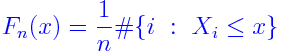

 . We want to compare
