Suppose that I toss a fair coin, and offer you Rs 10 for a head,
and demand $Rs 20$ for a tail. In other words, your gain (in Rs)
from this deal is $10$ for head and $-20$ for
tail. Both $10$ and $-20$ are constants, but since you
do not know which of these two constants you are going to get,
you gain is a variable. Since it varies with chance, we call it
a random variable.
Notice that here we have a function from $\{head,~tail\}$
to $\{10,-20\}$ defined as
$$\begin{eqnarray*}
head & \mapsto & 10,\\
tail & \mapsto & -20.
\end{eqnarray*}$$
There is nothing random about this function. The randomness comes
from mechanism that decides what gois into this: head or tail?
We use this idea to define random variables mathematically. We
start with a random experiment which is the provider of the
randomness. Then any function defined on its sample space is
called a random variable. To be precise, it is the function
(which is not at all random) that is called the random
variable. Thus, if in the above coin toss example, we replace the
fair coin with a biased coin, but keep the payment rules the
same, then we still have the same random variable.
Beginners often find it odd: a random variable is neither random
nor a variable!
However, it is not as unnatural as it sounds. In calculus also we
write $y = x^2$ and say $y$ is a variable as well
as $y$ is a function of $x.$
EXAMPLE:
In the coin tossing example with a fair coin, let your gain be
denoted by $X.$ (or sometimes $X(w)$, if you want to emphasize
that it is a function). Find $P(X=10).$
SOLUTION:
The immediate answer is $\frac 12.$ Let's see the steps that led
to this answer. $P(X=10)$ is the probability that $X$
is $10,$ i.e., the probability that the coin toss has
produced an outcome for which the function $X$ takes the
value $10.$ Thus
$$
P(X=10) = P\big\{w\in\{head,tail\}~:~X(w)=10\big\}.
$$
Now $\big\{w\in\{head,tail\}~:~X(w)=10\big\} = \{head\},$ and so
the problem now reduces to finding $P(\{head\}),$ which is $\frac 12.$
The general case, then, looks like this: We have a random
experiment with sample space $\Omega.$ A random
variable $X$ is a function $X:\Omega\rightarrow S$
where $S$ is any codomain of our choice. If some one gives
us some $A\subseteq S$ and asks us to find $P(X\in A),$ we
are to actually find
$$
P\big(\big\{w\in\Omega~:~X(w)\in A\big\}\big).
$$
Remember that this is the definition of $P(X\in A).$
The complicated looking set $\big\{w\in\Omega~:~X(w)\in A\big\}$ is
often abbreviated to $\{X\in A\}$ or $X ^{-1} (A).$
Earlier we had
talked about "good" sets and "bad" sets. What if someone asks us
to find $P(X\in A),$ where $X ^{-1} (A)$ is a "bad"
subset of $\Omega?$ Well, the answer is: We shall
simply refuse to find $P(X\in A)$ for such an $A.$ We shall
call such an $A$ a "bad" subset of $S$
(w.r.t. this $X$). A subset $A\subseteq S$ is "good" or
"bad" according as $X ^{-1} (A)$ is "good" or "bad" in $\Omega.$
EXAMPLE:
A fair die is rolled. I shall pay you Rs 10 if the die shows an
even number, you'll pay me Rs 20 otherwise. Again, let's denote
by $X$ your gain (in Rs). Express $X$ as a function
(as codomain you can take ${\mathbb R}$ or ${\mathbb C}$ or ${\mathbb Z}$
or $\{10,-20\}$ or any other superset of $\{10,-20\}$).
Let $A = \{10\}.$ Find $X ^{-1} (A)$ and using it
find $P(X\in A).$
SOLUTION:
Here $X ^{-1}(A) = \{2,4,6\}.$ So $P(X=10) = P(\{2,4,6\}) = \frac 16+\frac 16+\frac 16 = \frac 12.$
In each of these examples we had a random variable $X$ that
took only two values $10$ and $-20.$ Which $X$ do
you think is more profitable for you? Well, both are actually the
same so far as profit goes. Understand this carefully: the two
different $X$'s are completely different as functions (their
domains are also different), but in terms of the behaviour of the
output of the functions they are identical. This behaviour is
called the distribution of the random variable. It is the
distribution which we care about mostly in real applications. So
we often start a discussion as
Let $X$ be a random variable taking values $10$
and $-20$ each with probability $\frac 12.$
We understand implicitly that there is some random experiment (say
the coin toss experiment or the die roll experiment or something
similar) and some function from its sample space
to $\{10,-20\}$ such that the distribution is as
specified. In this
course, we shall often omit the sample space or
the function.
Sometimes we need to combine the values of two or more random
variables. Say $X,Y$ are both random variables and we want
to compute $X+Y.$ Since random variables are actually
functions, so this sum can be formed only when $X$
and $Y$ have the same domain. This simple point sometimes
needs careful handling as the following example shows.
EXAMPLE:
I am playing against two gamblers simultaneosly. One gambler
tosses a fair coin and pays Rs 10 for a head and takes Rs 20 for a
tail. The other gambler takes Rs 3 from me, rolls a fair die and pays me as many
rupees as the outcome. What is my total gain?
SOLUTION:
If I call the gain
from the first gambler $X,$ then $X$ is a function
from $\{head,tail\}$ to ${\mathbb R},$ while the gain from the
second gambler is a function $Y:\{1,2,3,4,5,6\}\rightarrow{\mathbb R}.$
Obviously, $X+Y$ does not make any sense here. We need to
first combine the two random experiments to get the product
sample space: $\{head,tail\}\times\{1,2,3,4,5,6\}$ and then
consider $X,Y$ both as functions from $\Omega$
to ${\mathbb R}.$ For example, $X(head,4) = 10$
and $Y(head,4) = 4-3 = 1.$
Now it is meaningful to talk about $X+Y.$
Depending on the distribution, a random variable may be of 3
types:
Discrete: These random variables take only countably
many (finite/infinitely many) values.
Continuous: If a random variable takes values in some
set $S$ such that $\forall a\in S~~P(X=a)=0,$ then we
call it a continuous random variable. Notice that
a continuous
random variable is not defined as a random variable that takes a
"continuous stretch of values". Howeever, most continuous random
variables do indeed take all values in an interval, e.g., height
of a randomly selected person.
Neither discrete nor continuous: These take
uncountably many values and for at least one value $a$ we
have $P(X=a)>0.$
In this course we shall focus on discrete random variables only.
The distribution of a discrete random variable is completely
specified by the countable set of values it can take, and the
probability with which it takes each of those values. These two
specifications together are called the probability mass
function (PMF) of the rv.
Any function of a random variable is again a random
variable. This is immediate from the definition of a random
variable (since composition of two functions is again a
function).
Notice that any function of a discrete random variable must again
be a discrete random variable.
Shall show
$$
\forall \epsilon>0 ~~ \exists M \in{\mathbb R} ~~ \forall x < M~~ |F(x)-0| < \epsilon.
$$
(Actually we may drop the absolute value sign around $F(x)$
since it is anyway $\geq 0$).
Take any $\epsilon>0.$
Let $A_n$ be the event that $\{X \leq -n\}$
for $n\in{\mathbb N}.$ Then $F(-n) = P(A_n).$
Clearly, $A_1\supseteq A_2\supseteq A_3\supseteq\cdots$
and $\cap A_n=\phi.$
So $P(A_n)\rightarrow 0,$ i.e., $F(-n)\rightarrow 0.$
So $N\in{\mathbb N} ~~F(-N)<\epsilon.$
Choose $M = -N.$
Take any $x < M.$
Then $0\leq F(x) \leq F(M)<\epsilon,$ since $F(\cdot)$ is nondecreasing.
So $|F(x)-0| < \epsilon,$ as required.
Shall show
$$
\forall \epsilon>0 ~~ \exists M \in{\mathbb R} ~~ \forall x > M~~ |F(x)-1| < \epsilon.
$$
(Actually we may drop the absolute value sign
around $|F(x)-1|$ is $1-F(x)$,
since $F(x)\leq 1,$ anyway.)
Take any $\epsilon>0.$
Let $A_n$ be the event that $\{X \leq n\}$
for $n\in{\mathbb N}.$ Then $P(A_n)=F(n).$
Clearly, $A_1\subseteq A_2\subseteq A_3\subseteq\cdots$
and $\cup A_n=\Omega.$
So $P(A_n)\rightarrow 1,$ i.e., $F(n)\rightarrow1.$
So $N\in{\mathbb N} ~~|F(N)-1|<\epsilon.$
Choose $M = N.$
Take any $x > M.$
Then $0\leq 1-F(x) \leq 1-F(M) <\epsilon,$ since $F(\cdot)$ is nondecreasing.
So $|F(x)-1| < \epsilon,$ as required.
Shall show:
$$
\forall a\in{\mathbb R}~~\forall \epsilon>0~~\exists \delta>0~~ \forall
x\in (a,a+\delta)~~|F(x)-F(a)| < \epsilon.
$$
Take any $a\in{\mathbb R}$ and any $\epsilon>0.$
Let $A_n$ be the event that $\left\{X\leq a+\frac 1n\right\}$ for $n\in{\mathbb N}.$
Also let $A$ be the event that $\{X\leq a\}.$
Try the rest yourself.
Then $A_1\supseteq A_2\supseteq\cdots$ and $\cap A_n = A.$
So $P(A_n)\rightarrow P(A)$ and hence $F\left(a+\frac 1n\right)\rightarrow F(a).$
Hence $\exists N\in{\mathbb N} ~~ |F\left(a+\frac 1N\right)-F(a)|<\epsilon.$
Choose $\delta = \frac 1N>0.$
Take any $x\in (a,a+\delta).$
Since $F(\cdot)$ is nondecreasing, hence $F(a)\leq F(x)
\leq F(a+\delta) < F(a)+ \epsilon.$
So $|F(a+x)-F(a)|<\epsilon,$ as required.
[QED]
A rather nontrivial theorem is that the converse is also
true. This converse is called the fundamental theorem of
probability.
Proof:Too technical for this course.[QED]
Proof:
Let $F:{\mathbb R}\rightarrow{\mathbb R}$ be nondecreasing and bounded from above.
Take any $a\in {\mathbb R}.$
We shall show that $\lim_{x\rightarrow a-} F(x)$ exists as a finite
number, i.e.,
$$
\exists\ell\in{\mathbb R}~~\forall \epsilon>0~~\exists \delta>0~~\forall x\in(a-\delta,a)~~|F(x)-\ell|\leq\epsilon.
$$
Consider the set $A=\{F(x)~:~x < a\}.$ Then $A\neq\phi$
and bounded from above (by $F(a)$).
So $\sup(A)\in{\mathbb R}.$
Choose $\ell = \sup(A).$
Take any $\epsilon>0.$
Then $\exists y < a~~F(y) > \ell-\epsilon.$
Choose $\delta = a-y > 0.$
Take any $x\in(a-\delta,a) = (y,a).$
Then $F(y)\leq F(x) \leq \ell,$ or, in other words, $\ell-\epsilon\leq F(x)\leq \ell.$
So $|F(x)-\ell|\leq \epsilon,$ as required.
[QED]
Proof:
Take any $a\in{\mathbb R}.$
Let $A = \{X < a\}$ and let $A_n
= \left\{X \leq a-\frac 1n\right\}$ for $n\in{\mathbb N}.$
Then $A_n\nearrow A.$
Hence $P(A_n)\rightarrow P(A).$
So $F\left(a-\frac 1n\right)\rightarrow P(A).$
But $F\left(a-\frac 1n\right)\rightarrow F(a-),$ since $F(a-)$ exists.
Hence $P(X < a) = F(a-),$ as required.
[QED]
Proof:
$P(X=a) = P(X\leq a)-P(X < a).$
[QED]
The following theorem justifies the adjective "continuous" for a
random variable.
There is no clear guideline as to the choice of the domain of the
PMF, except that it must be a superset of $\{x_1,x_2,...\}.$
If you take the domain to be a strict superset, then you define
the PMF as
$$
p(x) = \left\{\begin{array}{ll}p_i&\text{if }x=x_i\\0&\text{otherwise.}\end{array}\right..
$$
Clearly, $\sum p_i = 1$ and $\forall i~~p_i\geq 0.$ A
consequence of the fundamental theorem of probability is that for
any countable set $\{x_1,x_2,...\}$ and for any
sequence $(p_i)_i,$ for which $\forall i~~p_i\geq 0$
and $\sum p_i=1,$ there is a (discrete) random variable of
which the PMF is
$$
p(x) = \left\{\begin{array}{ll}p_i&\text{if }x=x_i\\0&\text{otherwise.}\end{array}\right..
$$
The CDF of a discrete random variable is like a step function.
For many random variables we see a striking example of
statistical regularity.
w = sample(6,1000,rep=T)
profit =c(-20,10,-20,10,-20,10)
X = profit[w]
avgX = cumsum(X)/(1:1000)
plot(avgX,ty='l')
In fact, it is this phenomenon that first let man to study
probability. If you run a gambling game a large number of time
the average profit becomes more and more stable. Gamblers wanted
to guess this stable value beforehand. They argued as follows:
If I play this game a large number of times (say $n$ times),
then
approximately $\frac n2$ times I should get $10$
and the remaining $\frac n2$ times I should get $-20.$ So
approximately my total gain would be approximately
$$
\frac n2\times 10 + \frac n2\times (-20).
$$
So the average would be approximately this divided by $n,$
i.e.,
$$
\frac 12\times 10 + \frac 12\times (-20) = -5.
$$
Indeed, this simple argument turns out to be remarkably
accurate. Gamblers could not understand why it becomes so
accurate as $n$ becomes large. But they used this formula to
find out what they could expect the random variable to do in the
long run.
There is a wierd point in the definition of $E(X).$
We are working with $\sum p_i x_i.$ But then why is the
condition on $\sum |p_i x_i|$? The reason for taking this absolute
value should be clear from our crash course on infinite series.
EXAMPLE:
Suppose I have a rv that takes values $-1,0$ and $1$
with probabilities $0.1, 0.5$ and $0.4,$ respectively.
What is $E(X^2)?$
SOLUTION:
Here $X^2$ is a new rv. Call it $Y,$ say. Then $Y$
takes values $0$ and $1$ with probabilities $0.5$
each.
So $E(Y) = \frac 12.$
Here is another technique to arrive at the same result.
$$
E(X^2) = 0.1\times (-1)^2 + 0.5\times 0^2 + 0.4\times 1^2 = 0.5.
$$
This technique is often easier because here we do not need to
find the distribution of $Y=X^2$ first. Both these
techniques will always give the same answer.
Proof:
If $X$ takes only finitely many values, then the result
follows from distributivity of multiplication over addition.
For the countably infinite case, the result follows from rearrangement
property of absolutely convergent series.
[QED]
Here $X\leq Y$ means
$$
\forall w\in\Omega~~X(w)\leq Y(w).
$$
An immediate consequence of the above theorems is the following
theorem.
The condition "$X$ always lies in $[a,b]$" may be
written as $P(X\in[a,b])=1.$
However, if $a\in{\mathbb R}$ is replaced by $\infty,$ then the
result fails, i.e., it is possible to have a random
variable $X$ that is always finite (any real-valued random
variable will do, since $\infty\not\in{\mathbb R}$) such
that $E(X)=\infty.$
EXAMPLE:
It is a standard fact that $\sum\frac{1}{n^2}<\infty.$ Let the
sum be $c.$ (The exact value of $c$
which is $\frac{\pi^2}{6},$ is of no importance here).
Then consider a random variable $X$ that takes values
in ${\mathbb N}$ and $P(X=n)=\frac{1}{cn^2}.$
Then $E(X) = \frac 1c\sum\frac 1n=\infty.$
By the way, if $X$ can take values $x_1,x_2,...$, there
is no guaranty that $E(X)$ will equal any of
the $x_i$'s. For example, if the $X$ is the outcome of
a fair die, then $E(X)=3.5,$ which is not a possible
outcome.
EXERCISE:
If $E(X) = \mu,$ then what is $E(X-\mu)?$
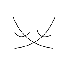
Next we shall need a new concept, that of a convex
function. Graphically, $f(x)$ is a convex function if its
graph is like a bowl opening upwards (possibly slanted). Some
examples are shown below.
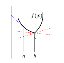
Mathematically we may define a convex function as follows.
While this definition is graphically quite intuitive, you
may have seen other definitions of convexity
elsewhere. Read here to learn more
about equivalences between different definitions of convexity.
In the following diagram the blue line is $\ell_a.$ Both the
red lines are candidates for $\ell_b.$
Proof:
Let $\mu = E(X).$ Consider $\ell_\mu(x)$ as mentioned
in the definition of convexity.
Since the graph of $\ell_\mu(x)$ is a straight line passing
through $(\mu,f(\mu)),$ hence it must be of the form
$$
\ell_\mu(x) = f(\mu)+m(x-\mu),~~x\in{\mathbb R}.
$$
So
$$
E(f(X)) \leq E(\ell_\mu(X)) = E(f(\mu))+mE(X-\mu) = f(\mu)+0 = f(E(X)),
$$
as required.
[QED]
EXERCISE:Which is larger $(E(X))^2$ or $E(X^2)?$ Assume
that both exist finitely.