If we want to combine values of different random variables (e.g.,
by addition, subtraction etc or comparison like $\leq$), then
they must be jointly distributed. If we have $n$ jointly
distributed real-valued random variables, then you may consider
them as components of an ${\mathbb R}^n$-valued random
variable. Sometimes we call such a random variable a multivariate
random variable, as opposed to a univariate one.
We shall now extend the various familiar concepts about ${\mathbb R}$-valued random
variables to ${\mathbb R}^n$-valued random variables.
The extension of the concept of discreteness is straightforward.
The definition of continuous random variable is slightly more
confusing. For ${\mathbb R}$-valued random variables we had two
equivalent definitions:
ever singleton set has probability zero,
CDF is continuous.
For an ${\mathbb R}^n$-valued random variable, these two conditions
are not equivalent (the latter is stronger). We use the stronger
condition as the defintion of continuity of
an ${\mathbb R}^n$-valued random variable.
Caution: Most books take a much stronger definition of
continuity for joint distribution. More precisely, that
definition should be called absolute continuity, which we
shall learn later.
The following example shows that the first condition is indeed
weaker than the second.
EXAMPLE:
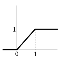
Consider the function with the following graph:
Clearly it satisfies the 4 conditions of being a CDF. Hence we
know that there is a random variable $X$ with this CDF (by
the fundamental theorem).
Define a ${\mathbb R}^2$-valued random variable
as $Y=(X,1).$ Show that for any $(a,b)\in{\mathbb R}^2$ we have $P(Y=(a,b))=0.$
Also show that the CDF of $Y$ is not continuous.
SOLUTION:
$P(Y=(a,b))= P(X=a~\&~1=b)\leq P(X=a)=0,$ since $X$ is
a continuous random variable.
Also, the joint CDF is
$$
F(a,b) = P(X\leq a~\&~1\leq b) = \left\{\begin{array}{ll}0&\text{if }b <
1\\F(a)&\text{if }b\geq 1.\\\end{array}\right.
$$
If we take $(a_n,b_n) =\left( \frac 12, 1-\frac 1n\right),$
then $(a_n,b_n)\rightarrow \left(\frac 12,1\right).$
Now $F(a_n,b_n)\equiv 0,$ and so $F(a_n,b_n)\rightarrow 0.$
But $F\left(\frac 12,1\right) = \frac 12\neq 0.$
If you are given two jointly distributed random
variables $X,Y$ and you know their joint distribution,
i.e. given any $A\subseteq{\mathbb R}^2$ you know $P((X,Y)\in A),$
then you can work out the probability distribution of $X$
and $Y$ separately from this, i.e., for any
fiven $B\subseteq{\mathbb R}$ you can find $P(X\in B)$ and $P(Y\in
B)$ as follows:
$P(X\in B) = P(X\in B~\&~ Y\in{\mathbb R}) = P((X,Y)\in A),$
where $A = B\times{\mathbb R}.$ Similarly, for $Y.$
The definition of expectation is straightforward extension of
the univariate case.
If $X$ is an ${\mathbb R}^n$-valued random variable,
and $h:{\mathbb R}^n\rightarrow {\mathbb R}^m$ is any function,
then $E(h(X))$ is defined component by component, and is said
to exists finitely iff all the component expectations exist finitely.
Proof:
In this course we shall prove this only when $X,Y$ are both
discrete random
variables.
First, notice that $X+Y$ is again discrete.
Because:
If $X$ takes values in the countable
set $\{x_1,x_2,...\}$ and $Y$ take values in the
countable set $\{y_1,y_2,...\},$ then each possible value
of $X+Y$ must be of the form $x_i+y_j.$ There are only
countably many such values.
Let $p_{ij} = P(X=x_i~\&~ Y=y_j).$
Then $P(X=x_i) = \sum_j p_{ij}$ and $P(Y=y_j) = \sum_i p_{ij}.$
So $E(X) = \sum_i x_i P(X=x_i) = \sum_i x_i \sum_j p_{ij},$
and $E(Y) = \sum_j y_j P(Y=y_j) = \sum_j y_j \sum_i p_{ij} .$
By the given condition both these series converges absolutely,
and may be grouped and arranged in any way without changing the
sum.
So $\sum_i\sum_j |x_i p_{ij}|< \infty,$ and $\sum_j\sum_i |y_j p_{ij}|< \infty.$
Now $|x_i+y_j|\leq |x_i|+|y_j|$ by triangle
inequality.
Hence $\sum_{i,j} |(x_i+y_j)p_{ij}| <\infty$ and
so $E(X+Y)$ exists finitely. Also
$$
E(X+Y) = \sum_{i,j} (x_i+y_j)p_{ij} = \sum_i\sum_j x_ip_{ij} +
\sum_j\sum_i y_jp_{ij} = E(X)+E(Y),
$$
as required.
[QED]
This result leads to simple trick that we discuss next.
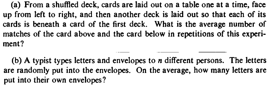
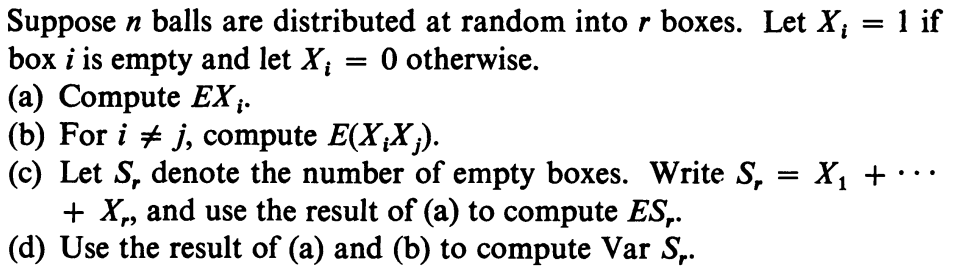
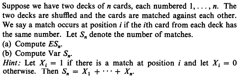
Suppose that you are to find expected number of something. For
example, $n$ letters are randomly put into $n$
addressed envelops, and you are to find $E(X),$
where $X$ is the number of correctly placed letters.
would you count $X$ In any given situation like the
following, you can find $X$ by first putting a check mark
for each correctly placed letter and then counting the total
number of check marks.
Mathematically each ckec mark is an indicator. For
example, the indicator for the $i$-th letter is
$$
I_i = \left\{\begin{array}{ll}1&\text{if }i\mbox{-th letter is placed correctly}\\0&\text{otherwise.}\end{array}\right..
$$
Counting the number of check marks amounts to
summing $I_i$'.s Thus, $X = \sum I_i.$
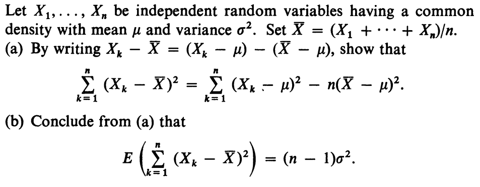
Notice that each $I_i$ is a random variable, and $E(X) = \sum E(I_i).$
Since each $I_i$ takes only the values $1$
and $0,$ hence $E(I_i) = P(I_i=1).$
Now $I_i=1$ means $i$-th letter has been placed
correctly. This is has probability $\frac{(n-1)!}{n!} = \frac 1n.$
So $E(X) = n\times \frac 1n = 1.$
It's a bit surprising that $E(X)$ does not depend on $n.$
An important special case of jointly distributed random variables
is that of independent random variables. To state the definition
we shall intriduce a new terminology: If $X:\Omega\rightarrow S$ is
a random variable, then by "an event in terms of $X$" we
shall mean $\{w\in\Omega~:~ X(w)\in A\}$ for some $A\in
S.$ Similarly, if $X:\Omega\rightarrow S$ and $Y:\Omega\rightarrow
T$ are jointly distributed random
variables, then "an event in terms of $X,Y$" means
$\{w\in\Omega~:~ (X(w),Y(w))\in A\},$ where $A\subseteq S\times T.$
EXAMPLE:
If $X,Y,Z$ are independent random variables, then
$$
P(X^2+Y^2 \leq 4~\&~ Z\neq 5) = P(X^2+Y^2 \leq 4)P(Z\neq 5).
$$
Proof:
Split $\{1,...,n\}$ into two disjoint
subsets $\{i_1,...,i_k\}$ and $\{j_1,...,j_{n-k}\}.$
Let $Y = f(X_{i_1,...,i_k})$ and $Z =
g(X_{j_1,...,j_{n-k}}),$ where $f,g$ are any two
functions.
Take any two sets $A,B.$ Then
$$P(Y\in A~\&~Z\in B) =
P(f(X_{i_1,...,i_k})\in
A~\&~g(X_{j_1,...,j_{n-k}})\in B) =
P(f(X_{i_1,...,i_k})\in A)P(g(X_{j_1,...,j_{n-k}})\in B) = P(Y\in
A)P(Z\in B).
$$
[QED]
Proof:Immediate from the definition of independence.[QED]
Proof:Immediate from the definition of independence.[QED]
Proof:
We shall prove this for the case where $X,Y$ are both
discrete (hence so is $(X,Y)$).
Let $p(x,y), p_X(x)$ and $p_Y(y)$ be the joint and
marginal PMFs, respectively.
Then
$$
E(XY) = \sum_{x,y} xy p(x,y) = \sum_{x,y} xy p_X(x)p_Y(y) =
\sum_x x p_X(x)\times \sum _y yp_Y(y) = E(X)E(Y).
$$
The grouping and rearranging were justified since the series were
absolutely convergent.
[QED]
Proof:
The first part follows immediately from the fact that $E(XY)=E(X)E(Y).$
A counter example for the second part is as follows.
$X$ takes values $-1,0,1$ with equal
probabilities. $Y = |X|.$ Direct computation
shows $E(X)=E(XY)=0$ and so $cov(X,Y)=0.$
But $P(X=0~\&~Y=1) = 0 \neq P(X=0)P(Y=1).$
[QED]
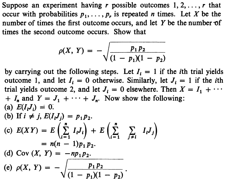
The $cov(\cdot,\cdot)$ function behaves much like ordinary
multiplication. The following theorems show this.
Also we have
EXAMPLE:
The analog of $(a+b)^2 = a^2+2ab+b^2$ here is $V(X+Y) =
V(X)+2 cov(X,Y) +V(Y).$ This also shows that if $X,Y$ are
independent, then $V(X+Y) = V(X)+V(Y).$
Proof:
The result is obvious if $X$ is degenerate. So let's
consider the case where $X$ is not degenerate. Then $V(X)>0.$
Define $Z = Y-\underbrace{\frac{cov(X,Y)}{V(X)}}_\beta X.$
We know that $V(Z)\geq 0.$
Now,
$$
V(Z) = V(Y) + V(\beta X) - 2cov(Y,\beta X) = V(Y) + \beta^2 V(X)
- 2 \beta cov(X,Y).
$$
Since $\beta = \frac{cov(X,Y)}{V(X)},$ this reduces to
$$
V(Y) - \frac{cov(X,Y)^2}{V(X)}.
$$
Since this is $\geq0,$ the inequality follows immediately.
Also equality holds iff $V(Z)=0$, i.e., $Z$ is degenerate.
So we have $V(X) X - cov(X,Y) Y = kV(X)$ for some $k\in{\mathbb R}.$
This completes the proof.
[QED]
By Cauchy-Scwartz inequality, $rho(X,Y) \in [-1,1].$ Also,
$\rho(X,Y)=-1$ or $\rho(X,Y)=1$ if and only
if $X,Y$ are linearly linearly related with probability 1,
i.e., $\exists a,b,c\in{\mathbb R}$ such that $P(aX+bY=c)=1.$