








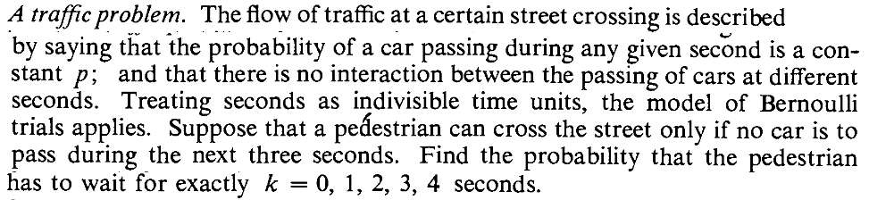

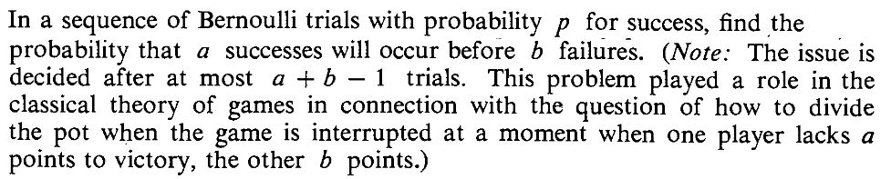

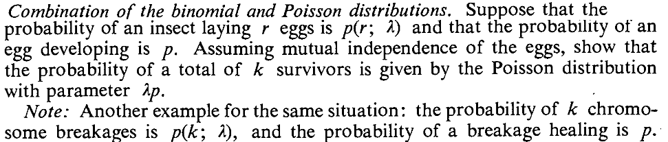
| Some people (including those who created the R software) use a slightly different convention. For them the number of '$0$'s preceding the first '$1$' is a Geometric random variable. |
barplot(dgeom(0:10, prob=0.5))In R each distribution has a short name. It is
geom
for the Geometric distribution. For each distribution there are 4
functions in R: these are formed by appending the
prefixes d, p, q
and r before the short name. The d
prefix gives the PMF, e.g., dgeom. The
prefix p gives the CDF,
e.g., pgeom. The prefix q gives the
"inverse" of the CDF, also called the quantile
function. Finally, the r prefix generates random
number from the distribution.
data = rgeom(1000, prob=0.5)
table(data)
barplot(table(data))
Where used: Suppose that we have a Bern$(\theta)$ random experiment. Let us perform the experiment again and again independently until we obtain the first `1'. Then count the total number of experiments you have done (among these all but the last one have produced outcome `0'.) The total number of experiments performed is a random variable with Geom$(\theta)$ distribution. Let us derive the PMF using the above description. Suppose that we have a coin with $P(head)=\theta.$ We keep on tossing it until we get the first head. Suppose that the first head comes at the $x$-th toss. Then the first $x-1$ tosses are all tails: $$ \underbrace{TT\cdots TT}_{x-1}H $$ Each of these tails occurs with probability $(1-\theta)$ and the final head occurs with probability $\theta.$ So the probability of having the first head at the $x$-th toss is $$ \underbrace{(1-\theta)\times\cdots\times(1-\theta)}_{x-1}\times \theta = (1-\theta)^{x-1} \theta, $$ which is the Geom$(\theta)$ PMF
EXAMPLE: If $X\sim$Geom$(0.3),$ find $P(X>2).$
SOLUTION: $$\begin{eqnarray*} P(X>2) &=& 1-P(X\leq 2)\\ &=& 1-\left(P(X=1) + P(X=2)\right)\\ &=& 1-(1-0.3)^{1-1}0.3 - (1-0.3)^{2-1}0.3\\ &=& 1-0.3-0.21 = 0.49. \end{eqnarray*}$$ ///EXERCISE: If $G$ is a Geom$(0.2)$ random variable, then compute the following probabilities.
EXERCISE: Find $P(T\mbox{ is even})$ where $T\sim$Geom$(0.4).$
Hint:
You will need the geometric series here. $$\begin{eqnarray*}P(X\mbox{ is even})&=& P(X=2)+P(X=4)+\cdots\\ &=&(1-\theta)\theta +(1-\theta)^3 \theta+ (1-\theta)^5 \theta+\cdots\\ &=& \theta(1-\theta)\left[ 1+(1-\theta)^2 + (1-\theta)^4+\cdots\right]. \end{eqnarray*}$$
EXAMPLE: Some versions of Ludo require you to get a `6' on the die before your counter can move. Sometimes it takes frustratingly long time before you finally roll a `6'. Let $X$ denote the number of rolls required to get the first `6'. If we assume the die is fair (i.e., each side has probability 1/6 of turning up), then what is the distribution of $X?$
SOLUTION: $X$ is a Geom(1/6) random variable. ///EXERCISE: In the above example compute the probability of getting the first `6' within the first 3 rolls.
EXERCISE: Some couples are so keen about having a son that they go on producing babies until they get their first son, and then they stop having children. Assume that at each birth a baby of either gender is equally likely. Also assume that the births are independent. Compute the probability that such a couple has exactly 2 daughters.
Hint:
Let $D$ denote the number of daughters. Then notice that $D+1$ is a Geom(0.5) random variable.Expectation and variance: If $X$ is a Geom$(\theta)$ random variable, then $$\begin{eqnarray*} E(X)& =& 1/\theta\\Var(X)& =& (1-\theta)/\theta^2. \end{eqnarray*}$$ $$\begin{eqnarray*} E(X) &=& \sum_{x=1}^\infty x(1-\theta)^{x-1}\theta\\ &=& \theta \sum_{x=1}^\infty x(1-\theta)^{x-1}\\ &=& \theta\cdot\frac1{(1-(1-\theta))^2}\\ &=& \frac{\theta}{\theta^2} = \frac1{\theta} \end{eqnarray*}$$ $$\begin{eqnarray*} E(X(X-1)) &=& \sum_{x=1}^\infty x(x-1)P(X=x) \\ &=& \sum_{x=1}^\infty x(x-1)(1-\theta)^{x-1}\theta \end{eqnarray*}$$ The term corresponding to `$x=1$' is zero. So we can as well start the sum from $x=2.$ $$\begin{eqnarray*} \sum_{x=1}^\infty x(x-1)(1-\theta)^{x-1}\theta &=& \sum_{x=2}^\infty x(x-1)(1-\theta)^{x-1}\theta \\ &=& \theta(1-\theta)\sum_{x=2}^\infty x(x-1)(1-\theta)^{x-2} \\ &=& \theta(1-\theta)\frac2{(1-(1-\theta))^3}\\ &=& \frac{2\theta(1-\theta)}{\theta^3} \\ &=& \frac{2(1-\theta)}{\theta^2} \end{eqnarray*}$$ $$\begin{eqnarray*} E(X^2) &=& E(X(X-1)) + E(X) \\ &=& \frac{2(1-\theta)}{\theta^2} + \frac1{\theta} \\ &=& \frac2{\theta^2} - \frac1{\theta} \end{eqnarray*}$$ $$\begin{eqnarray*} Var(X) &=& E(X^2) - (E(X))^2 \\ &=& \frac2{\theta^2} - \frac1\theta - \left(\frac1\theta\right)^2\\ &=& \frac{1-\theta}{\theta^2} \end{eqnarray*}$$
EXERCISE: Find the mean and standard deviation of a Geom$(\theta)$ random variable for the following values of $\theta.$
EXAMPLE: When a computer tries to connect to another computer, it sends a connection request to the second. Depending on how busy the second computer is, this request may be honoured (and so the connection is established) or refused (hence connection is not established.) In the latter case, the first computer waits for some time, and sends the same request again. In this way the first computer keeps on trying until connection is established. If the attempts are independent and if the probability of a refusal at each attempt is 0.2, then what is the expected number of attempts?
SOLUTION: If $X$ denotes the number of attempts required then $X$ is a Geom$(0.8)$ random variable. So $$ E(X) = 1/0.8 = 1.25 $$ ///EXERCISE: Compute $E(D)$ and $Var(D)$ in the son-daughter exercise above.
EXERCISE: If $X$ follows NegBin$(3,\frac14)$ distribution, find the following probabilities.
EXERCISE: $Y\sim$NegBin$(r,\theta).$ Compute $E(Y)$ and $Var(Y)$ for the following values of $r$ and $\theta.$
EXERCISE: Using the above result and the mean and variance of Geom$(\theta),$ derive the formula for mean and variance of NegBin$(r,\theta).$
Hint:
Use the result that $E(X_1+\cdots+X_r)= E(X_1)+\cdots+E(X_r).$ Also, since $X_1,...,X_r$ are independent, so $Var(X_1+\cdots+X_r)= Var(X_1)+\cdots+Var(X_r).$It is also possible to derive these directly without using the Geometric distribution. The direct proof is more complicated and uses the result $$ {x-1\choose r-1} = (-1)^{x-r} {r\choose x-r}, $$ which is proved in the appendix.
barplot(dnbinom(0:10, size=3, prob=0.5))
EXERCISE: If $X\sim$Poi$(3),$ then find the following probabilities.
EXERCISE: What is the probability that a Poi$(5)$ random variable is even?
Where used: One use of Poisson distribution is in approximating Binomial distribution.EXAMPLE: $X$ has Bin(1000,0.01) distribution. Compute $P(X=5)$ approximately by using Poisson approximation.
SOLUTION: Here $n=1000$ and $\lambda = 0.01.$ So we should take $\lambda = 1000\times 0.01 = 10.$ By Poisson approximation, $X$ is approximately a Poi(10) random variable. Hence $$ P(X=5)\approx e^{-10}10^{5}/5! = 0.03783. $$ It is instructive to compare this with the exact value, which is $$ P(X=5) = {1000\choose 5} (0.01)^5(1-0.01)^{1000-5} = 0.03745. $$ ///EXERCISE: A box has 100 items, each of which either passes a quality control test (OK) or fails the test (BAD). If a box has more than 3 BAD items, then the box is rejected by the quality control inspector. It is known that each item is OK with probability 0.01, and that the items are independent. Use Poisson approximation to compute the probability that a box is not rejected.
Expectation and variance: If $X$ has Poi$(\lambda)$ distribution then $$\begin{eqnarray*} E(X)&=&\lambda\\ Var(X)& =& \lambda. \end{eqnarray*}$$ $$\begin{eqnarray*} E(X) &=& \sum_{x=0}^\infty xP(X=x)\\ &=& \sum_{x=0}^\infty x\frac{e^{-\lambda}\lambda^x}{x!}\\ \end{eqnarray*}$$ The term for `$x=0$' is zero in this sum. So we can drop it to get $$\begin{eqnarray*} \sum_{x=0}^\infty x\frac{e^{-\lambda}\lambda^x}{x!} &=& \sum_{x=1}^\infty x\frac{e^{-\lambda}\lambda^x}{x!}\\ &=& e^{-\lambda}\sum_{x=1}^\infty x\frac{\lambda^x}{x!}\\ &=& e^{-\lambda}\sum_{x=1}^\infty \frac{\lambda^x}{(x-1)!}\\ \end{eqnarray*}$$ Now put $y=x-1.$ $$\begin{eqnarray*} e^{-\lambda}\sum_{x=1}^\infty \frac{\lambda^x}{(x-1)!} &=& e^{-\lambda}\sum_{y=0}^\infty \frac{\lambda^{y+1}}{y!}\\ &=& e^{-\lambda}\lambda\sum_{y=0}^\infty \frac{\lambda^{y}}{y!}\\ &=& e^{-\lambda}\lambda e^\lambda\\ &=& \lambda. \end{eqnarray*}$$ $$\begin{eqnarray*} E(X(X-1))&=& \sum_{x=0}^\infty x(x-1)P(X=x)\\ &=& \sum_{x=0}^\infty x(x-1)\frac{e^{-\lambda}\lambda^x}{x!}\\ \end{eqnarray*}$$ Drop the first two terms (which are both zeroes) to obtain $$\begin{eqnarray*} \sum_{x=0}^\infty x(x-1)\frac{e^{-\lambda}\lambda^x}{x!} &=& \sum_{x=2}^\infty x(x-1)\frac{e^{-\lambda}\lambda^x}{x!}\\ &=& e^{-\lambda}\sum_{x=2}^\infty x(x-1)\frac{\lambda^x}{x!}\\ &=& e^{-\lambda}\sum_{x=2}^\infty \frac{\lambda^x}{(x-2)!}\\ \end{eqnarray*}$$ Substitute $y=x-2$ to see that $$\begin{eqnarray*} e^{-\lambda}\sum_{x=2}^\infty \frac{\lambda^x}{(x-2)!} &=& e^{-\lambda}\sum_{y=0}^\infty \frac{\lambda^{y+2}}{y!}\\ &=& e^{-\lambda}\lambda^2\sum_{y=0}^\infty \frac{\lambda^{y}}{y!}\\ &=& e^{-\lambda}\lambda^2 e^\lambda\\ &=& \lambda^2.\\ \end{eqnarray*}$$ $$\begin{eqnarray*} E(X^2) &=& E(X(X-1)+E(X)\\ &=& \lambda^2 +\lambda. \end{eqnarray*}$$ $$\begin{eqnarray*} Var(X) &=& E(X^2) - (E(X))^2\\ &=& \lambda^2 +\lambda - \lambda^2\\ &=& \lambda. \end{eqnarray*}$$EXERCISE: Find the expected values of the following random variables.
EXERCISE: Find the variance of a Poi$(\lambda)$ random variable for the following values of $\lambda.$
EXERCISE: If $X_1,X_2,X_3,X_4$ are independent random variables with distributions Poi(1),Poi(2),Poi(4) and Poi(5), respectively. Find the distribution of $(X_1+\cdots+X_4).$
Proof: Clearly, $X+Y$ takes non-negative integer values.
Let $k$ be any such value. Then $$\begin{eqnarray*} P(X+Y = k) &= & P\left(\cup_0^k \{X=i~\& Y=k-i\}\right)\\ &= & \sum_0^kP( X=i~\& Y=k-i)~~\left[\mbox{$\because$ disjoint}\right]\\ &= & \sum_0^kP( X=i)P(Y=k-i)~~\left[\mbox{$\because$ independent}\right]\\ &= & \sum_0^k \frac{ e^{-\lambda} \lambda^i}{i !}\times \frac{e^{-\mu} \mu^{k-i}}{(k-i)!}\\ &= & \sum_0^k \frac{ e^{-(\lambda+\mu)}}{i! (k-i)!} \times \lambda^i \mu^{k-i}\\ &= & \sum_0^k \frac{ e^{-(\lambda+\mu)}}{k!} \times \binom{k}{i}\lambda^i \mu^{k-i}\\ &= & \frac{ e^{-(\lambda+\mu)}}{k!} \times \sum_0^k \binom{k}{i}\lambda^i \mu^{k-i}\\ &= & \frac{ e^{-(\lambda+\mu)}}{k!} \times (\lambda+\mu)^k, \end{eqnarray*}$$ as required. [QED]Proof: Since $p = \frac \lambda n,$ hence $$ \binom{n}{k} p^k (1-p)^{n-k} = \frac{n! }{k!(n-k)! }\times \frac{\lambda^k}{n^k}\times \left(1-\frac \lambda n \right)^{n-k}. $$ Separate out all factors free of $n$ to rewrite this as $$ \frac{ \lambda^k}{k!} \times \frac{ n! }{(n-k)! n^k }\left(1-\frac \lambda n \right)^{n-k}. $$ Now $$ \left(1-\frac \lambda n \right)^{-k}\rightarrow 1, $$ since $k$ is fixed. Also and $$ \left(1-\frac \lambda n \right)^n \rightarrow e^{-\lambda}. $$ Finally, since $k$ is fixed, we have $$ \frac{ n(n-1)\cdots(n-k+1) }{ n^k }\rightarrow 1, $$ completing the proof. [QED]