Date: Apr, 2014

[Update:[Sat Apr 26 IST 2014]]

Associating copulas with a vine

So far we have defined a vine as an abstract mathematical object: a sequence of nested trees. There is no concept of probability in it. Now we shall bring that in.

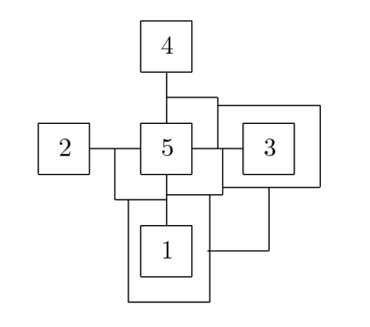
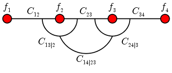
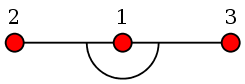
Let V be a regular vine. We associate a univariate density with each of the variables. These densities may be chosen completely arbitrarily. Also with each edge we associate a bivariate copula with density. Thus for the following vine we have specified 4 univariate densities and 6 bivariate copulas:

Notice how we have labelled the copulas using conditioned and conditioning sets.

A theorem by Bedford and Cooke (2001), which deserves to be called the fundamental theorem of vines, basically states that for any such choice there is a unique joint distribution of the variables such that the univariate desntities are the marginals and for each edge ij | D the copula of the conditional distribution of X_i, X_j given X_D is C_ij|D.

Two points are to be noted about this theorem, one positive and one negative.

The positive point

How may bivariate copulas do you need to specifiy the dependence structure completely for n variables? As many as there are edges in the vine. The lowest level tree has n-1 edges, the next higher level tree has n-2 edges, and so on, up to the highest level tree, which has just 1 edge. So the total number of edges is

(n-1)+(n-2)+...+1 = n(n-1)/2,

which is n choose 2. There is one simple (but wrong) way of interpreting this: for n variables we are specifiying the bivariate copulas of all n choose 2 pairs of variables. While this would also require specification of the same number of bivariate copulas, but then the choices of tje copulas will not remain arbitrary. For example suppose that we specify a copula for ( X₁ , X₂ ) that forces X₁ < X₂ with probability 1. Similarly we can specify a copula for ( X₂ , X₃ ) which forces X₂ < X₃ with probability 1. Obviously, we cannot specify a copula for ( X₁ , X₃ ) that forces X₃ < X₁ with probability 1.

Thus a vine may be considered as a clever way of arranging the dependence that allows each copula to deal with a separate part of the dependence. This may be compared to the way a basis generates a vector space, the span of each vector remaining separate.

The negative point

The theorem above has a somewhat technical condition whose need may not be readily apparent: we require all the copulas to have densities. Otherwise the theorem may fail as seen in the following counterexample:

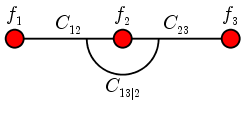
Suppose that we have th following vine:

Let us take each f_i to be Unif(0,1) and C₁₂ and C₂₃ to be the minimum copula, ie,

C₁₂ (x,y) = C₂₃ (x,y) = min { x,y } for x,y∈[0,1].

Also we take C_13|2 to be the indepdendence copula

C_13|2 (x,y) = xy for x,y∈[0,1].

The minimum copulas force X₁ = X₂ = X₃. Yet the indepdendence copula wants X₁ and X₃ to the indepdendent, which is impossible as X₁ and X₃ have nondegenerate distirbutions.

However, this does not violate the fundamental theorem, because the minimum copula does not have a density (wrt bivariate Lebesgue measure).

Vine copula density

The fundamental theorem guarantees the unique existence of a joint distribution. In fact, this joint distribution also has a density (wrt n-dimensional Lebesgue measure). It is possible to write down the density in a neat way:

f₁ × ··· × f_n ∏ c_ij|D ( F_i|D , F_j|D ),

where the product is taken over all edges of the regular vine. The typical edge is denoted by ij|D. Here c_ij|D is the copula density for this edge. Also F_i|D is the conditional cdf of X_i given X_D.

Why is the funadamental theorem true?

The proof of the fundamental theorem is notationally cumbersome. However one can see why it should be true using the following vine.

Here we have 4 variables. Let the joint density be g₁₂₃₄. Then we know that

g₁₂₃₄ = g₁ × g_2|1 × g_3|12 × g_4|123 .

We shall show that the vine (together with the marginals and copulas) unqiely determine all the densities in the rhs:

g₁ is nothing but f₁.
Sklar's theorem tells us that a joint distribution is uniquely determined by the marginals and the copula. We are given f₁, f₂ and C₁₂. So we get the joint distribution of X₁ and X₂. From this we can compute the conditional density of X₂ given X₁. So we have g_2|1.
Proceeding as above we can also obtain g_1|2. Similarly we can get g_3|2. Now consider the joint distribution of X₁ , X₂ given X₃. This is a bivariate distribution, and so is uniquely specified by the marginals: g_1|2 and g_2|3 and the copula C_13|2. Thus we get g_13|2, and from this we get g_3|12.
Similarly, we can find g_4|123. Make sure you see how!

Two special regular vines

A vine is a nested sequence of trees. Each tree can be of a different sturctures leding to a complicated vine. There are two special extreme cases that usually easier to handle. These are called C-vine and D-vine.

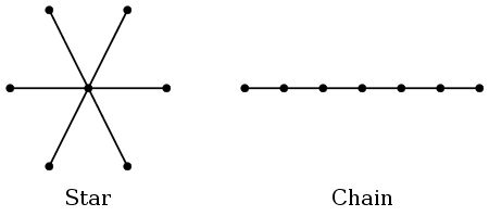
To learn about these we have to recall that a tree means a connected acyclic graph. Two extreme types of trees are the following:

You may think of the star configuration as the maximum connectivity case, and the chain configuration as the minimum connectivity case.

If all the trees in a vine are of the star type, then the vine is called a C-vine. If all the trees are of the chain type, then it is a D-vine.

There are standard ways to labelling the variables in a C-vine and a D-vine. We shall learn about these now.

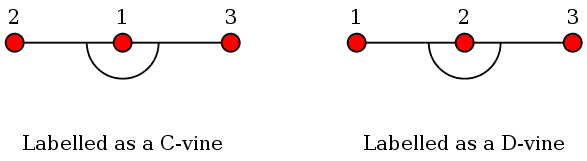
Notice that a tree of the star type has a centre. For a C-vine we label the variables in a way such that the lowest level tree has centre 1, the next tree has centre {1,2}, the next higher has { {1,2} , {1,3} }, etc.

For a D-vine the labelling is simpler. Just label the variables in the order of the lowest level tree.

Here is are two examples. Both examples show the same vine, which happens to be both a C-vine as well as a D-vine. But the labellings are different:

Simulation from a vine

One way to utilise a model is to simulate data from it. Simulating rom a vine is a tricky job. It is easiest for a C-vine, less easy for a D-vine, and quite complicated for a general regular vine.

Let us understand the basic idea first. If we are given a bivariate distribution of (X,Y), then one way to simulate from it is to generate from a marginal of X, and then generate from the conditional distribution of Y given X. Each random number generation starts with a Unif(0,1) random variable. So the bivariate generation requires two Unif(0,1) random numbers? A moment's thought should convince you that these must be indepdendent for (X,Y) to have the required bivariate distribution.

Now consider three random variables X,Y,Z. We shall first generate X, then Y given X. But finally we shall generate Z given X. So we shall need three Unif(0,1) random numbers, U,V,W, say. By the bivariate discussion we know that U,V must be indepdendent, and so must be U,W. But what about V and W? They do not need to be indepdendent. In fact, by allowing them to depend on each other we can introduce conditional dependence between Y and Z given X.

This is precisely the idea behind simulation from a C-vine. Let's take this C-vine:

To simplify the notation we shall assume that the marginals are all Unif(0,1). Then we proceed as follows.

First generate U₁ from Unif(0,1). Take X₁ = U₁.
Then generate U₁₂ from Unif(0,1) and use it to generate U₂ from U₁. Take X₂ = U₂.
Then generate U_23|1 from Unif(0,1), and use it to generate U₁₃ from U₁₂.
Use this U₁₃ to generate U₃ from U₁. Let X₃ = U₃.

It is a good exercise to write down the proof that this procedure indeed produces the correct joint distribution.

Another good exercise is to convince yourself that the same procedure fails if you label the same vine as a D-vine. This illustrates the additional difficulty involved in simulating from a D-vine.

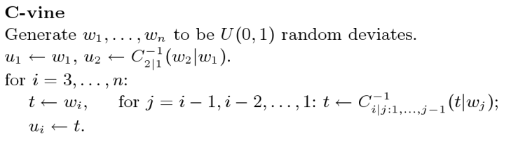
Here is the general algorithm for simulating from a C-vine. It is taken from chapter 7 of the book Dependence Modelling: Vine Copula Handbook:

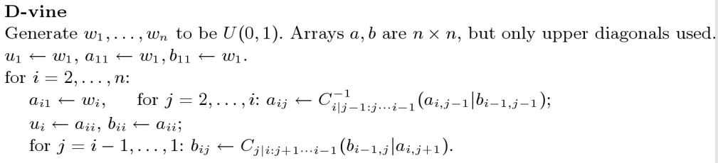
The general algorithm for simulating from a D-vine is more complex:

Fitting a vine to real data

A statistical model is a family of distributions, and is useless unless there is some way to select a member of the family that fits a given data set. Unfortunatley, fitting a vine is not a trivial task. This involves two things:

Choosing a vine structure
Estimating parameters to the associated copulas.

No best approach is yet known for choosing a vine structure. Here is a method by Kurowicka that uses a top-down approach. Thhe basic idea is to account for the strong dependences in the lower level trees, leaving only the weak one for the upper level trees. Kurowicka's approach seeks to measure the dependence strength using partial correlation. Let's explain using an example. Consider a data set with 5 variables. The first step is to compute the correlation matrix. Suppose it turns out to be the following.


A =
matrix(c(1,2,4,5,7,2,1,3,6,7,4,3,1,8,5,5,6,8,1,8,7,7,5,8,1),5,5)/10
diag(A) = 1
rownames(A)=colnames(A)=1:5
A
     [,1] [,2] [,3] [,4] [,5]
[1,]  1.0  0.2  0.4  0.5  0.7
[2,]  0.2  1.0  0.3  0.6  0.7
[3,]  0.4  0.3  1.0  0.8  0.5
[4,]  0.5  0.6  0.8  1.0  0.8
[5,]  0.7  0.7  0.5  0.8  1.0

We have to convert it to the partial correlation matrix. This is basically just inverting the matrix and then "normalising" the inverse. Here normalising means: Treat the inverse as a convariance matrix, and compute the corresponding correlation matrix. The following R function will do the normalisation.


normalise = function(mat) {
  inv=solve(mat)
  D=diag(inv)
  M=diag(sqrt(1/D))
  ans=M %*% inv %*% M
  dimnames(ans)=dimnames(mat)
  ans
}

In our case the partial correlation matrix is


normalise(A)
            1           2           3          5
1  1.00000000  0.56578947 -0.04253482 -0.7658001
2  0.56578947  1.00000000  0.04253482 -0.7862960
3 -0.04253482  0.04253482  1.00000000 -0.2409305
5 -0.76580010 -0.78629597 -0.24093047  1.0000000
> normalise(A)
           1           2           3          4          5
1  1.0000000  0.53086537 -0.20335111  0.2245833 -0.7436613
2  0.5308654  1.00000000  0.09143354 -0.0827344 -0.6020940
3 -0.2033511  0.09143354  1.00000000 -0.7930315  0.3236372
4  0.2245833 -0.08273440 -0.79303146  1.0000000 -0.5612747
5 -0.7436613 -0.60209401  0.32363716 -0.5612747  1.0000000

Now look for the weakest dependence, ie, the partial correlation closest to zero. Here it is -0.0827344. It is the partial correlation between X₂ and X₄ given the rest. From this we get the highest level tree, which has a single edge with conditioned set {2,4} and conditioning set {1,3,5}.

Next we look for the two edges in the next lower level tree. One of the edgs must have {2, something} as the conditioned set, where something ∈ {1,3,5}. The conditioning set is {1,3,5} \ {something}. So the question is: how to find that something? Notice that X₄ plays no role here. So we focus attention on the remaining variables, and apply the same technique:


normalise(A[-4,-4])    
            1           2           3          5
1  1.00000000  0.56578947 -0.04253482 -0.7658001
2  0.56578947  1.00000000  0.04253482 -0.7862960
3 -0.04253482  0.04253482  1.00000000 -0.2409305
5 -0.76580010 -0.78629597 -0.24093047  1.0000000

Look for the minimum absolute value in the row of X₂. It is 0.04253482, and occurs in the column corresponding to X₃. So the something we were looking for is 3. Thus we get the edge 23|15.

Proceed similarly for the other edge. Here we focus attention on all the variables except X₂:


normalise(A[-2,-2])
           1          3          4          5
1  1.0000000 -0.2984810  0.3179254 -0.6266796
3 -0.2984810  1.0000000 -0.7914843  0.4762897
4  0.3179254 -0.7914843  1.0000000 -0.7680004
5 -0.6266796  0.4762897 -0.7680004  1.0000000

Look for the minimum absolute value in the row of X₄ (which, by the way, is not the 4-th row). The least absolute value is 0.3179254, and occurs in the column corresponding to X₁. So we get the edge 41|35.

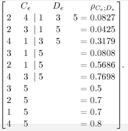
Proceeding thus, we get the following regular vine:

It is neither a C-vine nor a D-vine. Pictorially, it looks like this:

Estimating parameters

After we choose a vine (plus copulas and marginals with unknown parameters) we need to estimate these parameters based on data. As a joint distribution specified using vine-copula has a density, we can always apply MLE. This may not be computationally trivial. As may be expected, C-vines are easiest to deal with. The details are given in here. See section 3.7 starting on page 25. For this course it is enough to read from page 25 to page 29 up to (and excluding) inference for D-vines.

Comment Box is loading comments...