Statistics heavily relies on the availability of probability
distributions to model various observed features of a data
set. Many such distributions are available for univariate
data. But for multivariate data multinormal distribution used to
be the only useful distribution for a long time.
Copulas provide a rich family of multivariate
distributions. Indeed, it allows to combine univariate marginals
in arbitrary way. Sklar's theorem guarantees that any
multivariate distribution may be obtained like this. But still it
has one great problem: given a multivariate data set with
dimension >2 how to choose a copula that captures the
salient features of the data set? The main problem is that we
human beings cannot see any feature in a data set of
dimension >2. So it would help to have a technique to
design a copula by considering two variables at a time. And vine
is just a way to do that.
We shall start explaining the concept of vine starting with a
mathematical structure that apparently has no relation with
statistics. We shall need a definition from graph theory:
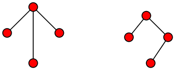
Typical examples are
These are trees on 4 vertices
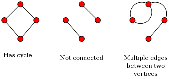
But the following two diagrams are not trees:
These are not trees
It is easy to see (and not difficult to prove) that any tree
on n vertices has exactly n-1 edges.
We shall now define a vine as a set of trees built in a
hierarchical manner. We shall start with a set
of n variables:
X1 , ... , Xn .
Consider them as n vertices and create a tree by joining
them with n-1 edges. It does not matter how you do this,
as long as you satisfy the conditions of a tree. Here is one
example:
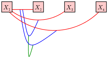
You could of course have proceeded in a different way, like the following, for example:
Another vine on 4 variables
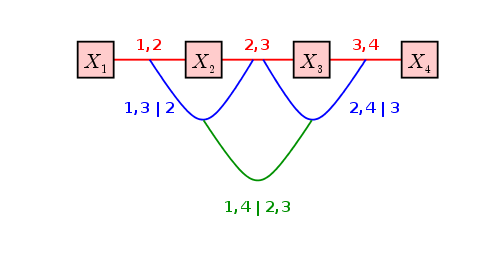
We have used different colours for the edeges of the different
trees. Mathematically the role of colour is played by
the order. The red edges (the oes that are drawn first)
are called edges of order 0. The blue edges have
order 1, the green edge has order 2.
A vine on n variables is sometimes called
an n-dimensional vine. It will have
n-i-1 edges of order i for i=0,...,n-1.
As you can guess, there are many
vines possible for a given dimension. It turns out that a subset of "nice" vines is
enough for statistical purposes. These are called regular
vines. To understand the concept we need a new definition:
Now we can define a regular vine:
The literature deals almost exclusively with regular vines. Here
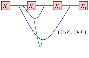
is an irregular vine, just as an object of curiosity:
An irregular vine: {{1,2},{3,4}}
connects {1,2} and {3,4} which are not neighbours as {1,2}∩{3,4}=φ
Naming the edges of a regular vine
Expressing an edge as a doubleton set is cumbersome. Fortunately,
there is an easier naming system available for regular vines. For
this we define two sets for each edge: the conditioned set
and the conditioning set. Let's start with an example:
Consider the edge {{1,2},{2,3}}, which is an edges of
order 1. Ignore all the braces to get a list:
1, 2, 2, 3.
The set of all elements that occur more than once in this list is
called the conditioning set. Here it is {2}. The remaining
elements (which occur exactly once each) consitute the
conditioned set: {1,3}.
As another example consider the 0-th order
edge {1,2}. Its conditioned set is {1,2} and
conditioning set is φ.
This intuitive description may be difficult to apply for larger
vines. So it's good to learn the formal definition, which starts
by defining a constraint set for an edge. Intuitively, it
is the union of the conditioning set and the conditioned set. The
formal definition is recursive:
Now we can define conditioned and conditioning sets as follows.
The conditioned set is defined as CONSTRAINT(e) minus the
conditioning set.
It is easy to see that the conditioning and conditioned sets are
disjoint. A key observation leading to their usefulness for
regular vines is that each edge is characterised by the
(conditioned, conditioning) pair. Also the conditioned set is
always a doubleton set. The size of the conditioning set equals
the order of the edge.
Here is the standard naming comvention for edges in a vine: If
an edge has conditioning set {4,5,6} and conditioned
set {1,3} then the edge is named
1,3 | 4,5,6 .
Edges of order 0 have empty conditioning sets, so they are
written without any vertical bar, like