Date: Feb 21, 2014

A taste of text mining with SVM

We want to see if SVM can computationally distinguish the writing of William Shakespeare from that of Arthur Conan Doyle. For this we have taken some haphazardly chosen passages from either author, and created a supervised data set in the file auth.txt.

String kernels

We load the data as well as the kernlab package:


library(kernlab)
source("auth.txt")

It is easy to apply SVM using the string kernel, which is called stringdot in R. It accepts a number of parameters. We have used just one: length. It is the length of the substrings to be used.


svp1 = ksvm(txt,lab,kernel='stringdot',kpar=list(length=2),C=10)

We have two fresh passages from the two authors for testing purposes.


predict(svp1,list(freshDoyle))
predict(svp1,list(freshShakes))

SVM correctly recognises the authors in both cases!

Let's play a bit more with the kernel. We can work with all substrings up to a given length. This variant of the string kernel is specifued by the type='boundrange' parameter of the stringdot kernel. Now length refers to the maximum length.


svp2 = ksvm(txt,lab,kernel='stringdot',kpar=list(type='boundrange',length=5),C=10)

predict(svp2,list(freshDoyle))
predict(svp2,list(freshShakes))

Even here the predictions are perfect.

Bag-of-words kernel

As we are dealing with human-readable texts here, a better alternative to string kernels is the bag-of-words kernel. Unfortunately, the kernlab package does not implement it out-of-the-box. So we shall need to write some code.

First let's familiarise ourselves with the R function strsplit that splits a given string into "words". If we want to use the space character as word boundary:


strsplit("To be or not to be",' ')

Output from R

[[1]]
[1] "To"  "be"  "or"  "not" "to"  "be"

We also need to break words at the punctuaions marks. Here is a first attempt to use both comman and space:


strsplit("a, b cd",', ')

Output from R

[[1]]
[1] "a"    "b cd"

Oops, that's not what we wanted! Here R just looks for the string ", ". We also want to allow a comma or a space to work separately. So we use the | operator, which stands for "or".


strsplit("a, b cd",',| ')

Some punctuaions are longer than a single character, e.g., a dash (--).


strsplit("The good-natured man said--OK",',| |--')

Here is pretty comprehensive list of a punctuations applied to the first passage in our data set.


strsplit(txt[[1]],' |,|!|?|.|"|:|;|--')

Next we have to create a frequency distribution:


table(strsplit(txt[[1]],'[ ,!?.":;]+|--'))

The frequency distribution is a just numeric vector where each entry is labelled with a word. R achieves such labelling via dimnames.


temp = table(strsplit(txt[[1]],'[ ,!?.":;]+|--'))
dimnames(temp)

We shall often need the set of words. So let's have a handy function for that:


wordsIn = function(b) dimnames(b)[[1]]

The following code snippet acheives two things: it extracts the frequency distribution for each passage in our sat set, and also creates the dictionary (the union of the sets of all the worlds in all the passages).


bag=NULL
full=c()
for(i in 1:length(txt)) {
  temp = table(strsplit(txt[[i]],' |,|!|?|.|"|:|;|--'))
  words = wordsIn(temp)
  words = words[words!=''] #To avoid words of length zero
  bag[[i]] = temp[words]
  full = union(full,words)
}

The line words = words[words!=''] avoids words with length zero. Such "words" are generated automatically when two word boundaries appear consecutively, eg, if the text is

She said-- Aha, nice!

Then R imagines an empty word between -- and the space following it, again between the comma and the following space.

Next we "lift" each frequency distribution to a frequency distribution over the full dictionary by assigning zero frequencies to the words not occuring in a passage.


dat = matrix(0,28,length(full)) #28 = number of passages in our data set.
colnames(dat) = full
for(i in 1:28) {
  dat[i,wordsIn(bag[[i]])] = bag[[i]]
}

A smart way to implement the bag-of-words would be to avoid explicit computation of φ, but we take the computationally inefficient route, which is easier to code:


phi = function(newText) {
  temp = table(strsplit(newText,' |,|!|?|.|"|:|;|--'))
  words = wordsIn(temp)
  words = words[words!='']

Nothing new so far. Now create an empty frequency distribution over the full dictionary.


  res = rep(0,length(full))
  names(res) = full

The new passage may contain words not in our "full" dictionary (which was constructed based on only the training data). We need to filter out such words. The intersect function is just the tool for this:


  commonWords = intersect(full,words)
  res[commonWords] = temp[commonWords]
  return(res)
}

Now we can use Euclidean inner product kernel (called vanilladot in kernlab):


svp3 = ksvm(dat,lab,type="C-svc",kernel='vanilladot',C=10)

Let's see how the predictions go for the two test cases:


predict(svp3,matrix(phi(freshDoyle),1))
predict(svp3,matrix(phi(freshShakes),1))

Both are correct!

k-nearest neighbour classification

A stark contrast with SVM, the k-nearest neighbour method of classification is little more than trivial common sense. Not that it always performs well (no method does, for that matter!), but its absolute simiplicity and ease of computation makes it a competitive alternative.

The idea is to have a metric on the feature space. Given any new case we find its k nearest neighbours (according to this metric) in the supervised data set (the actual number may increase in case of ties). We classify the new case by majority vote among these neighbours (resolving ties arbitrarily).

We shall employ this to recognise stars! This might sound like a useless academic example, but this is actually an important problem. Often multiple telescopes (usually situated in space) monitor the same part of the sky. To achieve greater information, the data sent by them need to be collated. So we need to come up with decision rules to make statements like:

This star in this data set is actually the same as that star in that data set!

Let's load the appropriate package:


library("class")

Here our training data set consists of 60 stars from the Hyades star cluster and 60 other stars.


trn = read.table("train.dat",head=T)
dim(trn)
names(trn)

We know that the first 60 are Hyades stars,


trueClass = c(rep("Hyad",60),rep("NonHyad",60))

Here are some test cases, stars whose membership in the Hyades star cluster is assumed unknown (actually we know that the first 28 of them belong to the Hyades star cluster, and the remaining 28 don't, but we shall see if k-NN method can find that).


tst = read.table("tst.dat",head=T)
dim(tst)

Finally we apply the method:


foundClass = knn(trn,tst,trueClass,k=3)

The prediction turns out to be correct every single time!

Unsupervsed classification techniques

Here we shall start with an unsupervised data set. We may or may not be told the number of classes (or clusters, as they are commonly called in the unsupervised scenario). A simple method is called the k-means method, which must not be confused with the k-nearest neighbours method of supervised classification.

k-means clustering

We shall first illustrate the priciple with a toy example. The necessary code is hidden in the file km.r. Don't peep inside th file right now. Just follow the discussion below. You can check out the contents of the R script file later.


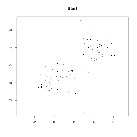
source('km.r')

val = startGame(sample(100,2))

You'll a get plot like this:

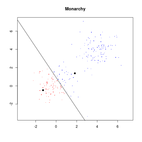
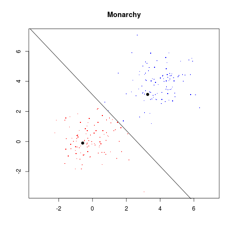
Two kings chosen randomly Here we have two clusters and we have chosen two random points to serve as "kings".

The algorithm proceeds by alternating two steps that we shall call Monarchy and Democracy. First we perform the Monarchy step, where the kings enlist all points nearest to them as their subjects.


val = monarchy(val)

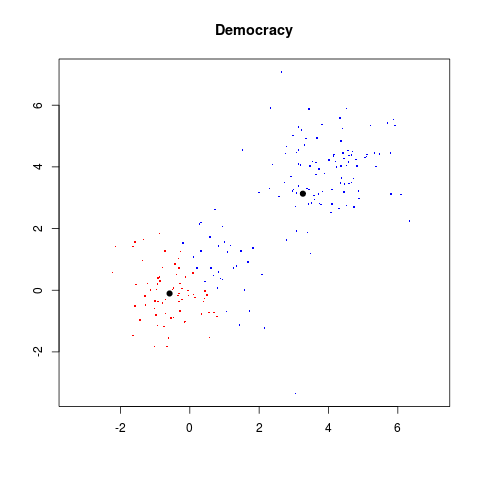
After Monarchy 1 Notice how we now have two kingdoms separated by the perpendicular bisector between the kings.

Next comes Democracy: the kings are abolished. The points of each country choose their leaders by taking average over the kingdom.


val = democracy(val)

After Democracy 1 But the Democracy is short-lived, as the leaders start behaving as kings, and start enlisting subjects.

After Monarchy 2 And the steps keep on alternating like this until Democracy and and Monarchy are hardly discernible from each other (somewhat like India?)!

Slideshow

This is the description of the 2-means algorithm (i.e. k-means algorithm with k=2). The method is similar for other values of k.

Satellite imaging with k-means

Here is a satellite image that I got from Google:

A satellite image If you can see two land masses amidst a sea, then what your brain has done is a simple clustering. It has clustered the pixels into two clusters: land and sea. We often need to do this automatically using a computer. Tese are useful for arial surveys, monitoring enemy territory etc.

What the satellite camera "sees" is just 3 numbers (red, green and blue) for each pixel. These are stored in the file sat.dat.


dat = read.table("sat.dat")

names(dat) = c("red","green","blue")

Let's reproduce the image first, just to make sure the data have been ingested correctly.


attach(dat)

mycol = rgb(red,green,blue,max=255)

rows = 1:75
columns = 1:40

z = matrix(1:3000,nrow=75)


image(rows,columns,z,col=mycol)

If you do not like to see axes and labels around the image:


image(rows,columns,z,col=mycol,
      bty="n",yaxt="n",xaxt="n",
      xlab="",ylab="")

A more statistical view may be had by making a 3D scatterplot.


library(scatterplot3d)


scatterplot3d(red,green,blue,color=mycol)

The scatterplot3d package produces quite dumb plots that cannot be interacted with. Try the rpanel package for 3D plots that can be rotated with the mouse.

Now we shall perform the k-means custering with k=2, say:


cl = kmeans(dat,2)

There are plenty of info packed in the output. We shall need only two:


names(cl)
cl$clus #which pixel is in which class

cl$center #the cluster centres

Let's convert the cluster centres into colours.


c2 = rgb(cl$cen[,1],cl$cen[,2],cl$cen[,3],max=255)

And then draw pixels in each cluster with the appropriate colour:


image(rows,columns, matrix(cl$clus,75,40),col=c2)

Wow! The land masses are clearly separated from the sea!

Want to zoom in on more details? Just increase k to 3:


cl = kmeans(dat,3)
c3 = rgb(cl$cen[,1],cl$cen[,2],cl$cen[,3],max=255)
image(rows,columns, matrix(cl$clus,75,40),col=c3)

More details are dded to the land msses, but the relatively uninteresting sea still remains a single cluster.

Comment Box is loading comments...



Click on next.