Date: Feb 19, 2014

SVM with non-numeric features

We have seen how the φ function maps the features into a (possibly higher dimensional) inner product space where the classes are linearly separable. This approach has another benefit: it allows SVM to be applied even to cases where the features are nonnumeric (eg, text strings).

String kernels

Example: Let x be a DNA sequence like

aagtctcccggga.

Consider a supervised classification data set consisitng of some DNA sequences classified into two classes.

tattcccgcaacttacgcca            trait A
gggaggtgacctaag                 trait A
 ...                             ...
ggcccccgcctgcacagtatgggcg       trait B
aggctgccgggttcacatgc            trait B

Here a typical feature is a DNA sequence. Notice that the sequences may be of different lengths. A simple way to compare two such sequences (of possible unequal lengths) is to reduce each string to the frequency distribution of the all substrings of length 2, say. Then any sequence is mapped to a numeric vector of size 4² = 16. We show two example below:

    ataat   gtacgtg
aa   1       0
at   2       0
ac   0       1
ag   0       0
 
ta   1       1
tt   0       0
tc   0       0
tg   0       1

ca   0       0
ct   0       0
cc   0       0
cg   0       1

ga   0       0
gt   0       2
gc   0       0
gg   0       0

We can consider this is as our φ : D → IR¹⁶ function, where D is the space of all DNA strings. If we use the usual inner product in IR¹⁶ then we get a kernel K(x,y) defined on D × D as

K(x,y) = φ(x)'φ(y).

For example we have

K(ataat, gtacgtg) = 1.

◼

This kernel is called a string kernel. Obvious variants include changing the string length, allowing all substrings up to a given length. One may also tweak the kernel to customise it for particular cases, e.g., using a weighted inner product in IR¹⁶ where longer substrings are given higher weights.

Bag-of-words kernel

In text mining one has to classify human-readable text documents into some classes (e.g. by topic). Then the bag-of-words kernel is a better approach than the string kernels. Here again we map the features (i.e., the text documents) to frequency distributions. But we consider whole words instead of substrings.

Example: Consider the two sentences:

x₁: to be or not to be that is the question.

and

x₂: please answer the question given below.

We first create a dictionary which is the set of all the words occuring in the two sentences:

{to, be, or, not, that, is, the, question, please, answer, given, below }

Now we get the two frequency distributions:

            to be or not that is the question please answer given below
x1:         2  2  1   1   1    1  1    1        0      0      0     0
x2:         0  0  0   0   0    0  1    1        1      1      1     1

Notice how we use a common dictionary so that the frequency vectors are all of the same length. ◼

Now we can define a bag-of-words kernel by taking a suitable inner product of the frequency vectors. Lots of customising options are available: weighting by length of the word, giving higher weights to proper nouns (starting with capitals), down-weighting commonly occuring words like "the", "a" etc. Indeed, the ease of incorporating heuristic tweakings is one of the main advantages of SVM.

Nominal features

Often a categorical variable is encoded numerically, where the numbers are used at a nominal level. For example, a variable called gender may take values 1 for Male and 2 for Female. Of course, it is meaningless to say that a Female is twice a Male! So performing SVM directly with these is not a good idea. We can suitably choose a φ function that maps the nominal values to numeric vectors meaningfully. For example, φ:{1,2}→ IR² may be

φ(1) = (1,0) and φ(2) = (0,1).

All possible subsets and ANOVA kernels

If the features are just sets of some symbols, then we can consider all possible subsets of the symbols, and consider the frequency distributions.

Example: Suppose we have our symbols are the 26 lowercase letters, and a feature is a subset like {a,x,m,u,e,r,d}. There are 2²⁶ possible subsets of the entire alphabet (counting the empty subset). We can count which of these subsets occur in our feature. Thus each feature is mapped to 2²⁶-dimensional vector of 0's and 1's (mostly 0's).

If you take the Euclidean inner product in this 2²⁶ dimensional vector space, then you get the all possible subsets kernel.

There are efficient ways to compute the kernel without explicitly computing φ. ◼

An easier (and more popular) variant is the so-called ANOVA kernel where we conider only subsets of a given size.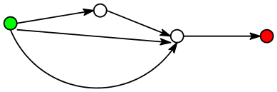

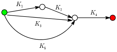
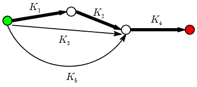
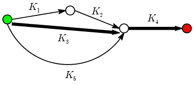
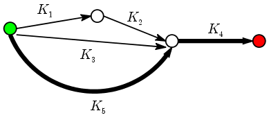
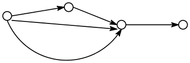
Graph kernels

A rich class of kernels (that subsumes all the above) is the class of graph kernels. Here we start with a finite directed acyclic graph (DAG). Thnk of this as a diagram like the one shown below.

It consists of some nodes connected by arrows. Multiple arrows are allowed between the same pair of nodes. The only restriction is that the arrows must not form a cycle (hence the term acyclic).

Claim: A finite DAG must have at least one node where no arrow ends, and at least one node from where no arrow starts.

Justification: Start from any node, and continue to follow random arrows. Due to the finite acyclic nature of the DAG, you cannot go on like this for ever. A node where you have to stop must be a node without any outgoing arrows. Similar arguement works for the other half of the claim.///

Pick any start node (i.e., a node with no incoming arrow) and also a terminal node (one without any outgoing arrow).

Start node shown in green, terminal node in red Label all the arrows with kernels of your choice (you may use the same kernel multiple times).

So now you have quite a complicated thing in your hand:

A finite DAG,
A start node (S)and a terminal node (T),
A kernel for each arrow.

Now we are ready to define a graph kernel: Given two features x,y we consider all the paths from S to T. For each path, apply to x,y all the kernels associated with the arrows along the path, and multiply them. So you get one number for each path. Add them up over all paths. That's the value of K(x,y).

In our example, we have 3 paths. The contributions of each path is shown below.

Contribution of this path: K₁(x,y) × K₂(x,y) × K₄(x,y)

Contribution of this path: K₃(x,y) × K₄(x,y)

Contribution of this path: K₅(x,y) × K₄(x,y) Adding all the contributions we get

K(x,y) = ( K₁(x,y) K₂(x,y) + K₃(x,y) + K₅(x,y) ) K₄(x,y).

There cannot possibly be any doubt as to the tremendous flexibility of this kernel. We have freedom to choose the DAG, the start and terminal nodes, and the kernels for each arrow. In fact, this sheer flexibility might appear to be its disadvantage: How to choose all this to achieve good classification in a given problem?

One possible answer to this question lies in the use of finite automata to recognise patterns. Roughly speaking these are directed graphs (often contain cycles) where you start from the start node, and follow the arrows according to some prescription based on the input that takes you to some terminal node. You classify the input according to the terminal node you arrive at. This approach works well if the input pattern is mathematically precise (e.g., syntax rule of programming languages). Graph kernels may be considered as an attempt to use the same approach allowing for some uncertainty.

Comment Box is loading comments...