So far we have dealt with only the linear case. A nonlinear
situation may be mapped to a linear case via a suitable function
Φ : IRd → H, where H is some (possibly
infinite dimensional) inner product space. One example if shown
in the animation below where d=2 and H =
IR2. Click on the button to linearise the scatterplot.
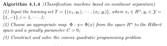
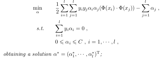
If we use such a transformation Φ then the algorithm
from the last lecture becomes
We notice that everywhere Φ is used only inside an
inner product. So instead of working with Φ we might as
well work with the function
K(x,y) = ( Φ(x) ċ Φ(y) ).
This function is called the kernel induced by Φ. As we
shall need to work with kernels a lot let's study them closely.
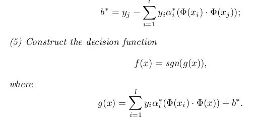
Kernels
All the excerpts below are from the main reference. First the definition:
Though we arrive at the concept of kernels via that of a
transfomation Φ, we always want to work the kernel
directly, because it is easier to work with than Φ. We
need some way to characterise
kernels directly (i.e., to be sure of the existence of a suitable
H and Φ without having to construct them
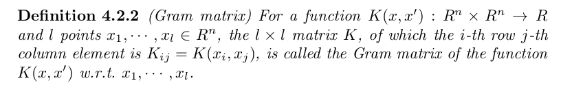
explicitly). For this we need the concept of a Gram matrix:
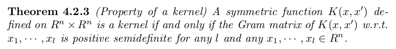
Here is a theorem that serves our purpose. We shall not prove
it. The proof is quite easy if H is finite dimensional.
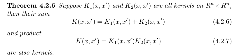
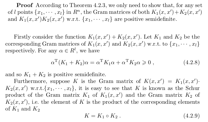
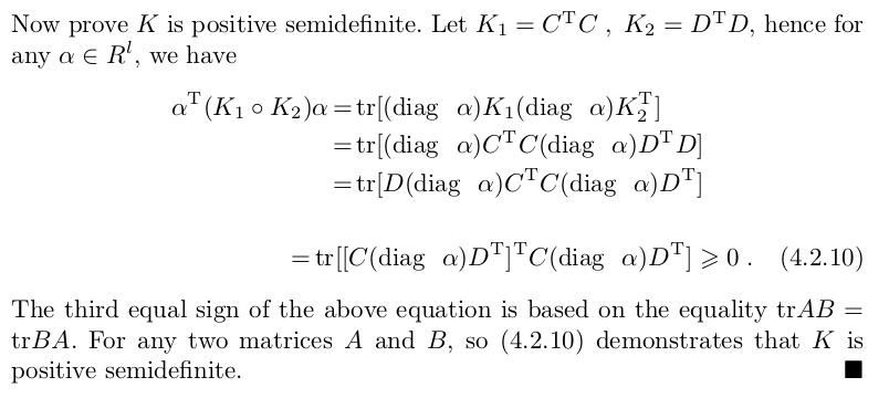
We shall often need to construct kernels satisfying various
conditions. This is facilitated by the fact the space of all
kernels is a closed under many useful operations. The following
theorems give some of them:
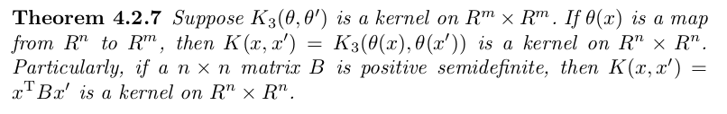
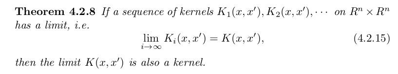
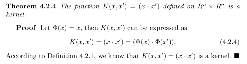
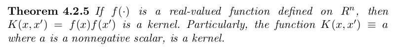
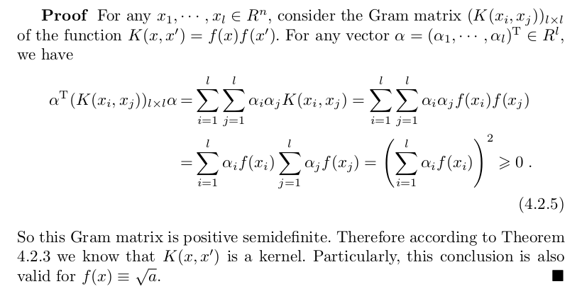
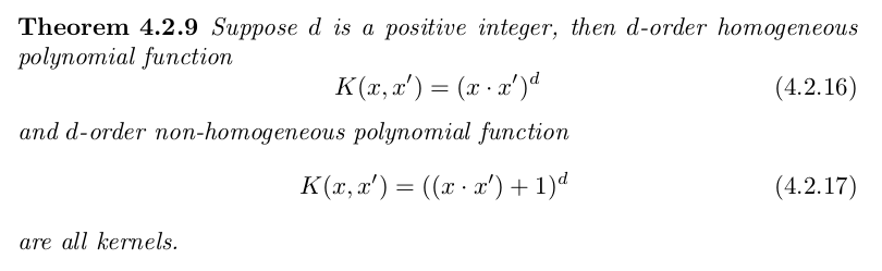
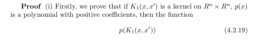
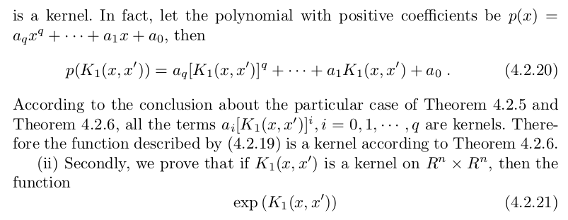
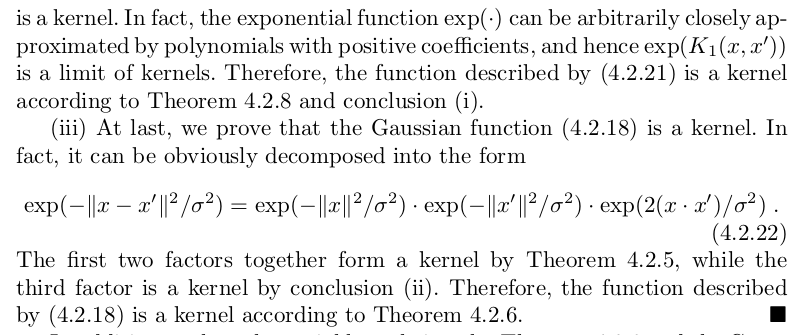
Next we need some simple kernels as basic building blocks. The
theorems below provide some such:
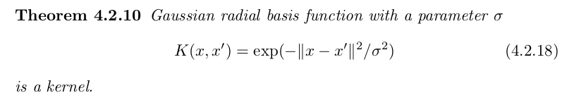
We can combine these using to create many different kernels. One
important example is the Gaussian Radial Basis Function (RBF) kernel: