Date: Feb 05, 2014

[Update:[Fri Feb 14 IST 2014]]

Space- and time-crunch

Multivariate statistics is a computation intensive branch of statistics. Unbearably slow computation and running out of space are nagging problems whenever we want to deal with large high dimensional data.

There are a number of popular ways out of these problems:

Modify the algorithm mathematically: We have already seen an example of this when we ran out of memory during PCA of the face data. There we performed eigenanalysis of YY' instead of the much larger Y'Y. We used the fact the nonzero eigenvalues are the same for both, and the corresponding eigenvectors are also related. Unfortunately, such tricks are not always available.
Use some lower level language: Languages like R or Matlab often add extra layers of bookkeeping and/or memory restrictions. So implementing a computation intensive algorithm in C is often a way out. But remember that most R packages are already written in C, and so if an R package runs too slow, then rewriting the algorithm in C may not help much.
Use harddrive-mapped RAM: This is a popular solution for space crunch. It makes the program run slower, but allows much larger data sets. The SAS software uses this technique very efficiently. Here the idea is that space crunch comes from shortage of RAM and not shortage of harddrive (you can easily add an external harddrive). If we keep our variables mostly in harddrive, and load only a small part of it into RM during each step of the computation, then we can by-pass the shortage of RAM. Of course, this calls for redesigning the algorithm so that only a small part of data is used in each step.
Parallel processing: This is a solution for time crunch. Modern CPU's are getting faster and cheaper. But the rate at which they are getting cheaper is more than the rate of getting faster. So it is easier to get 10 CPU's than one CPU that is 10 times faster. Parallel processing tries to get the benefit of the latter using the former. Parallel processing comes in two flavours:
- Distributed computing: Here we use a cluster of computers networked together. Each computer is a traditional one with a single CPU.
- Multicore processors: Here a single computer actually comes with multiple CPU's (eg, dual-core or 4-core etc).
A simple example is provided by the PCA face recognition problem. There we had to compute a large matrix product YY'. If we partition Y as
Y = [ Y₁ Y₂ Y₃ Y₄ Y₅ ]
then
YY' = ∑_i Y_i Y'_i
In the Map phase we can delegate the computation of each summand to a separate CPU, and perform the addition in the Reduce phase. There are many softwares to perform Map-Reduce. The most notable being HADOOP. It is a free software provided by Apache. R has a package that talks to HADOOP.

k-nearest neighbour method

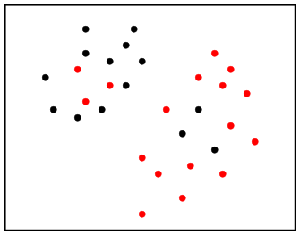
Consider a simple classification rule: given a fresh point x consider all the training points in its ε-neighbourhood and classify the new point by majority vote. Let's see the role of ε here. Take the data set:

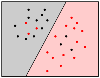
A typical ideal classification could be like this:

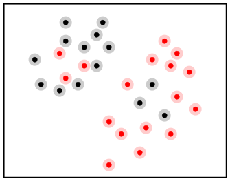
But if we use too small an ε, (say smaller than the smallest distance between two training points) then we shall get a classification like this. Each point forms an island of its own. If the new point lies outside all the islands, then our simple algorithm cannot even be applied! Obviously such an ε is a bad choice.

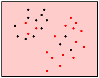
If we take ε too large, then the neighbourhood will contain all the training points. So we shall have only one class, the majority class.

Of course, we can avoid these bad extremes by choosing a medium-sized ε. Now consider the situation where the dimension is large. If we use Euclidean distance (d₂) then we have seen in the first class that the neighbourhood volume shrinks to 0. So we shall be in a situation like the first. If we use d_∞ distance, then the neighbourhood grows to ∞ in volume and so we end up being in the other extreme. Thus choice of ε as well as the metric becomes tricky as dimension grows.

A simple remedy is not to choose an ε beforehand, but to consider a neighbourhood (wrt d₂, say) just large enough to contain k training points. Here k is a tuning parameter. This approach is called the k-nearest neighbour method.

Support Vector Machine

Our main reference for this part is the book

Support Vector Machines Optimization Based Theory, Algorithms, and Extensions

Naiyang Deng,
Yingjie Tian
Chunhua Zhang.

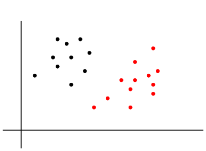
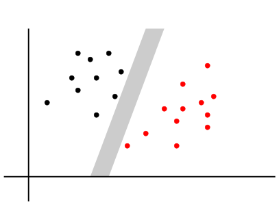
A softcopy may be downloaded here. We start with an example. Consider a bivariate case with just two classes as show below.

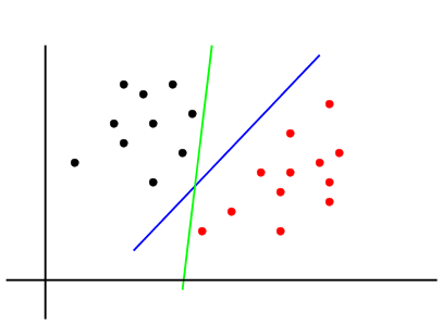
Two classes Clearly the classes can be separted by a line. There are infinitely mny such lines. We want to choose the "best". First we need to decide upon a definition for "best". Consider the two candidate lines shown below. Both separate the two classes. Intuitively, which one do you think is better?

Which line is the better separator? For the training data both are perfect, ie, the resubstotuion error is 0 for both. But imagine trying to classify fresh data. The green line is so close to the classes that a fresh point near a class may easily fall on the wrong side of the green line. But the blue line is farther away from both classes. Thus the blue one is better.

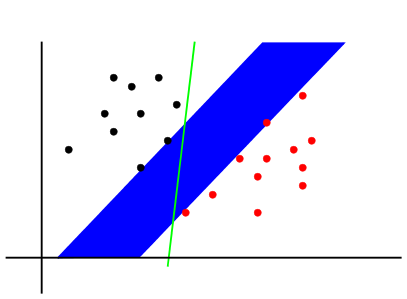
The fresh points (shown in grey) are misclassified by the green line. So one way to measure the "goodness of separation" by a line is to see how far the line is from training points of both the classes. It will help to think about wide strips instead of lines. The wider a strip the happier we are.

Wider strips provide better separation The blue strip above is wider than the green strip below.

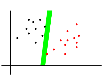
Narrower strips provide worse separation So instead of lines, let us now look for widest possible strips separating the training points from the two classes. Here is a a typical strip.

A typical (non-maximal) strip Obviously, this strip cannot be optimal, because it has not touched any point yet. So we can fatten it further:

A maximal strip (the best for its slope) When it hits at least one point on either side, we have achieved the best we can for strips of this slope. The points it hits on either side are called the support vectors. There could be more than one support vectors on either side.

So now we want to solve the optimisation problem:

Maximise width among all strips that separate the training points of the two classes.

We need to cast it in the language of mathematics before we can hope to solve this problem. This requires 3 steps:

Expressing a "strip" mathematically,
Finding the width in terms of our mathematical expression,
Expressing the condition that the strip separates the training points from the two classes.

Step 1: How to express a "strip" mathematically?

One way is by specifying the two boundaries, which are parallel lines. So we need to specify the common slope and the two intercepts. But since we want to allow the strip to be vertical (for which the slope is undefined), a better method is to use the form

w₁ x₁ + w₂ x₂ + b = 0.

for a line. Then we need to specify w_{1,w_2} for the common slope, and two values for b corresponding to the two boundaries. So 4 things are to be specified. We can reduce the number to 3 as follows. Let the two boundaries be

w₁ x₁ + w₂ x₂ + (b-1) = 0
w₁ x₁ + w₂ x₂ + (b+1) = 0.

Let's call the b-1 line the "positive" boundary, and the b+1 line the "negative" boundary. Convince yourself that any strip can be expressed like this uniquely, once it is decided which boundary is to be negative (or positive).

Example:If the positive boundary is y = x+10 and the negative boundary is y= x + 20, then write them as

y - x - 10 = 0,
y - x - 20 = 0.

Now divide them by 5 (to make the intercept difference come down to 2):

0.2 y - 0.2 x - 2 = 0,
0.2 y - 0.2 x - 4 = 0.

We need the positive boundary to have the smaller constant term, so change sign:

-0.2 y + 0.2 x + 2 = 0,
-0.2 y + 0.2 x + 4 = 0.

This may be expressed as

-0.2 y + 0.2 x + (3-1) = 0,
-0.2 y + 0.2 x + (3+1) = 0.

So we can take w₁ = -0.2, w₂ = 0.2 and b=3.◼

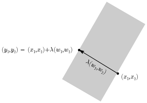
Step 2: Finding the width of strip given by (w,b)

The next step is to find the width of a strip given by w = ( w₁ , w₂ ) and b. For this we notice that if we draw a vector perpendicularly across the strip then it is along the direction of ( w₁ , w₂ ). Now take a point ( x₁ , x₂ ) on one boundary, say the negative boundary, and drop a perpendicular upon the other boundary. See the diagram below.

Finding the width of a strip The foot of the perpendicular satisfies the equation of the other boundry. If you do the computation, you'll see that ( x₁ , x₂ ) will cancel out, and you'll be left with a value for λ in terms of ( w₁ , w₂ ). (The number b will not play any role here.) A few simple steps will show that maximising the width is equivalent to minimising the length of ( w₁ , w₂ ).

Step 3: Express the separation condition

The final step is to mathematically express the condition: the strip separates the training points of the two classes. For this it will help to define a variable y which takes the value -1 for one class (the "negative" class, say), and 1 for the "positive" class. Thus y_i = -1 means the i-th training point is in the negative class, and y_i = 1 means that it is in the positive class. Then convince yourself that the condition

"all training points from the negative class are beyond the negative boundary of the strip, and all the training points from the positive class are beyond the positive boundary of the strip"

can be expressed as

∀ i
if y_i = 1 then (w₁ x_1i + w₂ x_2i + b) ≥ 1
and
if y_i = -1 then (w₁ x_1i + w₂ x_2i + b) ≤ 1

These two cases may be conveniently combined into a single condition:

∀ i y_i (w₁ x_1i + w₂ x_2i + b) ≥ 1.

Now that the three steps are over, our optimisation problem is that of finding ( w₁ , w₂ ) and b to

min w'w subject to ∀ i y_i (w₁ x_1i + w₂ x_2i + b) ≥ 1.

This is a quadratic programming problem and hence can be solved efficiently.

Hard and soft margin cases

So far we were assuming that the training points of the two classes were linearly separable (i.e., could be separated by a line). This is not the general case.

If we have such a situation then we have to allow strips that allows some points to cross boundaries, i.e., allowing

∀ i y_i (w₁ x_1i + w₂ x_2i + b) < 1.

Of course we do not allow this "too much". We measure the "badness" of the strip w.r.t. the i-th point by

(1 - y_i (w₁ x_1i + w₂ x_2i + b))₊ .

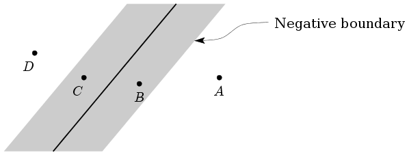
Consider the following diagram where we have shown 4 training points from the negative class.

Gradation of "badness" Point A is beyond the negative boundary of the strip, so nothing to worry about. Point B is on the correct side of the medial line of the strip (so it is correctly classified) but still we feel unhappy since it has come inside the strip. The cases for points C and D are even more serious, as both of them are misclassified. The case of D is the worst.

So we may now look for a strip that is wide as well as the total "badness" is low. As you can guess, these are qualities of opposing nature, and we have to look for a trade-off. Any such trade-off must start by bringing the two qualities on a common denominator (i.e., by answering a question like: How much badness are we willing to tolerate to increase the width by one unit?) For this we introduce a cost parameter C, and minimise

w'w + C ∑ (1 - y_i (w₁ x_1i + w₂ x_2i + b))₊ .

Also here we have to optimise over all strips. This is called soft margin SVM. As C increases we approach case discussed earlier: hard margin SVM.

Notice that even here we have a convex programming problem, and so have an efficient solution.

Comment Box is loading comments...