Model-based clustering

The idea

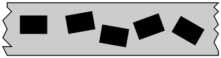
Computer vision is an important application area for clustering. Here the computer eye is a camera and we want to know about the "things" in its field of vision. This aim is acheivwd by clustering the pixels: This pixel belongs to a chair, that one to a table, and those belong to the background, and so on. A common scenario is where a robot counts / arranges items on a conveyer belt. Suppose that a manufacturing unit produces rectangular sheets and dumps them haphazardly on a conveyer belt. The belt passes under a suveilance camera which typically sees something like this:

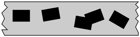
Here it is easy to see that there are 5 clusters, and hence 5 objects. Now suppose that the camera sees something like this:

Here there are only 4 clusters due to overlap. But still we can understand that there are actually 5 objects, since each object is known to be a rectangle. Utilising prior information about the shape of clusters while clustering is what is called model-based clustering. Thanks to this extra information, we can handle overlapping clusters.

The math

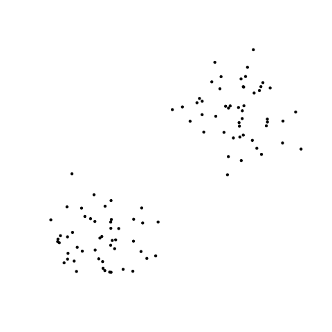
There are different ways to capture the idea of "shape" statistically. One possibility is to assume that a typical point in the data set comes from a mixture distribution. Thus, a data set that looks like this:

may be considered as coming from a mixture of two bivariate normal distributions. We can visualise the following model:

God (or Nature, if you are an atheist!) has two bivariate normal distributions up his sleeves.
He tosses a coin to pick on of them.
Then he generates (X,Y) from this distribution.
He repeats the entire exercise n times (each time starting with a fresh toss of the same coin).
Finally he reports only the generates ( X_i , Y_i )'s, but not the outcomes of the tosses.

You only know the above scheme, but not the parameters involved (the probability of head for the coin, or the parameters of the bivariate normals).

In this case finding the mle is not computationally very easy. So we employ the EM algorithm. We shall illustrate with a 1-dim example, where everything is as above, except that God uses two univariate Gaussian distributions. To simplify the exposition further we shall assume that the variances are known, 1 and 1/4. Also we shall assume that the coin is unbiased.

Thus we have

X₁ , ... , X_n ∼ 0.5 N(a, 1) + 0.5 N(b, 1/4).

Then likelihood function is

L(a,b) = const × ∏ [ 0.5 φ(X_i - a) + 0.5 φ(2(X_i - b)) ] .

Clearly, maximising this w.r.t. a,b is very difficult. Instead, first pretend that God actually gave us the outcomes of the coin tosses. Thus, our hypothetical data set becomes

( T_i , X_i ), i=1,...,n,

where

T_i ∼ Bern(0.5)

and X_i ∼ appropriate normal depending on value of T_i. Now the likelihood function is

L_comp (a,b) = 0.5ⁿ ∏₁ φ(X_i - a) ∏₂ φ(2(X_i - b)).

Here ∏₁ is over all cases where the coin showed Head and ∏₂ is over the remaining cases.

Taking log simplifies this considerably and prduces ℓ_comp (a,b). We would like to maximise this w.r.t. a,b, but unfortunately we really cannot compute ℓ_comp (a,b), as God actually did not tell us the T_i's.

What we shall do is to take conditional expectation of the ℓ_comp (·,·) function given only the X_i's, and maximise the conditional expectation.

Finding the conditional expectation is called the E-step, and maximising it is called the M-step of the EM algorithm.

The computation is pretty straightforward in our toy example, but gets messy when we work in multivariate situation with unknown variance matrices and more than two clusters.

The statistician can choose among a number of options trading generality with computational simplicity:

cluster proportions known/unknown?
each cluster has same/different variance matrix?
are the variance matrix constrained to be of special form (e.g., diagonal, compound symmetry etc)?

Comment Box is loading comments...