Date: Jan 24 2014

Visualising Mahalanobis's approach to LDA


#install.packages('deldir')
library(deldir)
x = rnorm(10)
y = rnorm(10)
deldir(x,y,plot=T,wline="tess")

Visualising Fisher's approach to LDA

We have already seen Fisher's approach in the last class. Click on the top left hand rectangle repeatedly to change the angle of projection.

The 1-dimensional projected points are shown below. The number shows the SSB/SSW ratio, which increases as separation of the two classes improve.

Though by no means essential to learning multivariate statistics, it is good to know how to produce an interactive animation like this in R. The R package tcltk is the main tool to use. The package rpanel is built on top of this, and is a bit easier to use, though does not always work. So we quickly show the steps involved in setting up an interactive graphical user interface (ie, an environment using buttons, sliders etc) using tcltk.

First a word about local and global assigments in R. Consider the following:


x = 3
f = function() {
  print(x)
  x = 5
  print(x)
}

x #Prints 3
f() #Prints 3 and then 5
x #Prints 3

If you run this, you'll see that initially x is 3 inside the function, but after the line x=5 it becomes 5. This is as expected. But after coming out of the function x reverts to its old value 3. Thus, any change made to x outside the function is visible inside the function as well, but the opposite is not true. So we call x=5 a local assignment.

Now compare this with the following:


x = 3
g = function() {
  print(x)
  x <<- 5  #This is the only difference from f() above
  print(x)
}

x #Prints 3
g() #Prints 3 and then 5
x #Prints 5

Now the change to x done inside the function is visible from outside the function as well. The line x <<- 5 is called a global assignment. Such assignments are important when different functions need to communicate with each other via global variables. We shall need them while using tcltk.

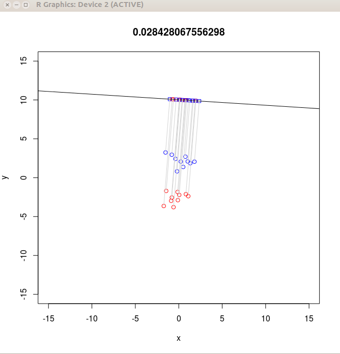
We are going to build something like the interactive animation shown above. Our final outcome will consist of two windows: a main plot window:

Plot window and a small control window:

Control window The control window has a slider to control the direction of projection. When you move it, the projection angle changes, and the plot is animated accordingly. The plot heading shows the value of the SSB/SSW ratio for the current projection. We shall now build this step by step.

In step 0, we design the entire thing. There are two parts, static and dynaic. The static part consists of the two classes shown in two colours. The dynamic part consists of the projection angle θ. The value of θ is specified by the control window, and is used to update the dynamics part of the plot (the moving lines, the changing heading). So much for the design.

In step 1 we shall tackle the static part. We encapsulate it in the following function:


genData = function() {
  y <<- c(rnorm(10,mean=-2.5), rnorm(10,mean=2.5))
  x <<- rnorm(20)
  n <<- length(x)
  colour <<- c(rep("red",10),rep("blue",10))

  data = cbind(x,y)

  T = 19* cov(data)

  W <<- 9*(cov(data[1:10,])+cov(data[11:20,]))
  B <<- T-W

  plot(data,xlim=c(-15,15),ylim=c(-15,15),col=colour)
}

Notice the global assignments used for variables that will be needed outside this function. Just invoke this function as


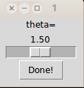
genData()

to see a plot containing only the static part.

In step 2 we shall create the control window to change θ . Remember that θ is the link between the control window and the main plot window. We shall need tcltk for this:


showWin = function() {
  require(tcltk)

  tt = tktoplevel() #This creates a blank the control window 

  laba = tklabel(tt,text="theta=") #A label saying "theta="

  

  tva <<- tclVar(1.5) #the variable theta 

  #Next we create the slider
  scla = tkscale(tt, command=doit, from=0.1, to=3, reso=0.01,
                     orient="horizontal", variable=tva)

  #and a button
  butt = tkbutton(tt,text="Done!", comm=function() tkdestroy(tt))

  #Finally put everything together
  tkpack(laba,scla,butt)
}

If you call this function like


showWin()

a little blank control window will be created, and you'll get an error message saying that doit is not available. This function, which we have called doit, is the main workhorse to dynamically update the plot using the changing value of θ .

In step 3 we shall write this function.


doit = function(...) {

The function starts by reading the value of θ from the control window. The control window always passes this value in an encoded way, so that we need to decode it first.


  theta = as.numeric(tclvalue(tva))

Next comes all the math required to draw the projections. They require little more than high school trignometry and coordinate geometry.


  cosTheta = cos(theta)
  sinTheta = sin(theta)
  r = 10

  a = r/sinTheta
  b = -cosTheta/sinTheta

  vec = c(sinTheta,-cosTheta)
  num = t(vec) %*% B %*% vec
  den = t(vec) %*% W %*% vec
  val = num/den

  b2p1 = b*b+1
  ab = a*b

  px = (x+b*y-ab)/b2p1

  py = a  + b * px

Now we make the plot. Notice that plot everything, both the static as well as the dynamic part, everytime.


  plot(x,y,main=val,xlim=c(-15,15),ylim=c(-15,15),col=colour)
  points(px,py,pch=22,col=colour)
  abline(a=a,b=b)

  for(i in 1:n)
    lines(c(x[i],px[i]),c(y[i],py[i]),col="lightgray")
}

Finally we need to invoke


showWin()

to get everything moving!

LDA in action

Today we shall apply LDA to banknote forgery detection. The data set is taken from Flury and Riedwyl (1988).

A Swiss 1000 Franc banknote We have 6 measurements on each of 100 genuine and 100 forged banknotes of the above type. We want to develop a classifcation rule to classify a banknote as genuine or forged based on these measurements.

First we load the data set.


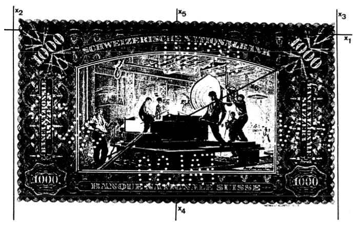
x = read.table('banknote.txt',head=T)
names(x)

We should never right into mathematics, before having a good look at the data first. Let's make a scatterplot matrix:


plot(x,col=x[,7]+1,pch='.')

Well, notice that the shapes of the clusters are sort of elliptical. Also the Diagonal variable has maximum discriminatory power. Top and Bottom put together also does a good job of discriminating. The pair Left nd Right also does a decent job. But Length is totally useless for discrimination.

Now let's see what LDA can do for us:


library(MASS)
fit1 = lda(Y~.,data=x)
fit1

Here is part of the output:


Coefficients of linear discriminants:
                  LD1
Length   -0.005011113
Left     -0.832432523
Right     0.848993093
Bottom    1.117335597
Top       1.178884468
Diagonal -1.556520967

Notice that the coefficient of Diagonal has the largest absolute value (which matches with the impression we got from the scatterplots: Diagonal has the maximum discriminatory power).

Next suppose that we have a new banknote with the following measurements:

Length=215.0, Left=130.2, Right=130.1, Bottom=9.5, Top=10.8, Diagonal=138.9.

We want to check if it is forged or not. The predict function will help us:


predict(fit1,list(Length=215.0,
                  Left=130.2,
                  Right=130.1,
                  Bottom=9.5,
                  Top=10.8,
                  Diagonal=138.9)) $ class

LDA requires the classes to all have the same Σ matrix. If this homoscedasticity assumption does not hold, then we may use Σ_i for the i-th class. This will lead to Quadratic Discriminant Analysis (QDA), which is also available in R:


fit2 = qda(Y~.,data=x)
fit2

Prediction is similar to LDA:


predict(fit2,list(Length=215.0,
                  Left=130.2,
                  Right=130.1,
                  Bottom=9.5,
                  Top=10.8,
                  Diagonal=138.9)) $ class

Overloading a function in R

You may be wondering how the same predict function could cope with both LDA and QDA. Actually, there are two functions behind the scene: predict.lda and predict.qda. Every object in R has a concept called class associated with it. It is just a string. The object returned by the lda function (which we called fit1) had class "lda". You can check it easily:


class(fit1)

When you call predict(fit1, etc ) then R first checked the class of fit1 and added that to the name of the function (and put a dot inbetween) to get "predict.lda", and this was the function that was actually called. Similarly for QDA


class(fit2) #returns "qda"

Indeed, you can assign whatever classes you want. For example, you can write


class(fit1) = "isi"

and then write


predict.isi = function (x) print("It works!")

Now calling


predict(fit1)

will print It works!

Cross validation

Given any supervised classification method an important question is "How well does it perform?" or "How close is our decision to the truth?" This is like teaching a class of students and asking how well they students have really learned the subject. Let us explore this student-teaching analogy. When a teacher starts to teach he has a set of problems (and their solutions) in mind that he wants his students to learn to solve after the course. Consider the following two strategies:

The teacher solves all these problems in class as worked out examples, and then asks some of those very questions inthe exam.
The teacher solves majority of those problems in class, and uses the rest for the exam. Thus the exam problems are similar, but not the sameas the woked out problems.

Which is a better strategy? The second one, because the first strategy encourages learning by rote. After all a student is supposed to learn how to solve a population of problems, not just the few specific sample problems solved in class!

The situation is similar in case of supervised classification. If there are 4 classes, you may consider this as an MCQ with 4 options.

The idea of splitting all the available data into two parts, and using one part to "train" and the other part to "test" is called cross validation. Of course, this should be done in a fair way, in the sense that both the "train" part nd the "test" part should represent the entire data. For example, while teaching integration, it must not be the case that all the worked out examples are from method of substtution, while all the exam problems are from partial fractions!

It is a good idea to use stratified sampling for splitting the data into two parts. Let's implement the idea for the banknote data. There are two strata: good notes and bad notes. We first work with the good notes.


indGood = rep(1:5,20)

Now we shall scramble this:


randPerm = sample(100,100)
indGood = indGood[randPerm]

Now indGood is a vector of length 100 with exactly 20 ones, 20 twos etc but all these are randomly distributed. Let's do the same thing for the bad notes:


indBad = rep(1:5,20)
randPerm = sample(100,100)
indBad = indBad[randPerm]

Now we combine these:


ind = c(indGood,indBad)

We shall use all the cases with ind=1 as the test cases, the rest being the training cases:


trn = x[ind!=1,]   # Worked out example
tst = x[ind==1,-7] # Exam problems
truth = x[ind==1,7] # Answer keys to exam problems

Now the teaching starts:


fit = lda(Y ~ . , data = trn )

Thus lda plays the role of the teacher, and fit is what the students learn. Now it is time for the exam:


pred = predict(fit , tst)$class

Here pred is the student's answer. e have to now compare this with the answer key:


mean(truth!=pred)

If we repeat the same procedure 5 times (each time choosing a different train-test partition) then we get 5-fold cross-validation (CV):


err = NULL
for(i in 1:5) {
  trn = x[ind!=i , ]
  tst = x[ind==i,-7]
  truth = x[ind==i,7]
  
  fit = qda(Y ~ . , data = trn )
  
  pred = predict ( fit , tst ) $ class
  err[i] = mean ( truth != pred )
}

mean(err)

This approach is very general, and can be used for any supervided classification method. For example,just replace lda with qda above to apply CV to QDA.

By the way, what we called "learning by rote" in the student-teaching analogy, is called overfitting in statistics. CV is a great way to avoid overfitting.

Comment Box is loading comments...