Date: Jan 22, 2014
Why do people collect multivariate data? Put in another way, the
question is: Why would one take multiple measurements about the
same object? The most common answer is: To learn about the nature
of the object. Learning about the nature of an object means
finding out which class it belongs.
For example, an interview candidate is asked many
questions to enable the interviewers to classify the candidate as
either "eligible" or ineligible".
Thus classification is the most important of multivariate
statistics.
Classification is of two types:
supervised
unsupervised
When a kid learns the alphabet she is shown the letters
(which are nothing but pictures to her) and the teacher tells her
the names of the letters. This is an example of supervised
classification. Now suppose the kid has grown up and visits
China for the first time in her life. At some place she sees the
following:
Of course, she cannot read, but she notices that some letters are
repeated. So she can at least pick up the unique letters. This is
an example of unsupervised classification.
The term discriminant analysis is a synonym for supervised
classification. The term clustering is used for
unsupervised classification.
Here are the two set ups:
Supervised classification :
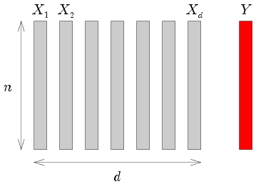
We have n items (say letters).
For each we have the same set of measurements:
X1 , X2 , ... , Xd .
Also we have a number of classes 1 , 2 , ... , c. For each
of the n items we are told the class to which it
belongs. Each item belongs to one and only one of the classes. So
our data set looks like
The Y vector gives you the classes. Our aim is to come up
with a classification rule so that any future case for which the
measurements are available may be
classified.
Unsupervised classification :
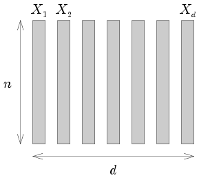
Here again we have n items (say letters).
For each we have the same set of measurements:
X1 , X2 , ... , Xd .
But that is all. In some cases we may also be told the number of
classes, but we have no idea about where the items belong.
So our data set looks like
Here our aim is twofold:
Identifying the classes,
Coming up with a classification rule to predict the classes
of future cases.
Usually the first is the more important aim.
As you can guess, the unsupervised case is harder than the
supervised one. All classification problems start as unsupervised
ones, because the measurements are the only real things, the
classes are imagined by us for ease of visualisation, just like
boundaries between countries. Supervised classification problems
are born in two ways:
Teacher-student: A botanist visits a new island and
finds many new kinds of plants. He classifies all these
plants. As he has never seen these plants before, it is an
unsupervised classification for him. After this is done he gives
new names to the classes he found. Now future students of botany
have to learn to recognise the name by looking at these
plants. For them it is a supervised classification.
Pattern recognition: A country is flooded with
counterfeit currency notes. The government can of course identify
a forged note using expensive detection machines. But ordinary
people are easily fooled. The way the government first detected
the forgery was an example of unsupervised classification, as the
government did not know how many (if any) forging techniques are
being used. But now the government wants to issue "An easy way to
recognise forgery" accessible to ordinary people. The easy way
should employ only measurements that can be made easily by the
ordinary people. So the government takes a bunch of good notes as
well as a bunch bad notes, makes those easy measurements on each,
and tries to see if there is a way to detect. This is an example
of supervised classification.
In our everyday life we meet the teacher-student type of
supervised classification more often. But in statistics the
pattern recognition scenario occurs more often. The same techniques
are used for both. However, the techniques for unsupervised
classification are quite different from the techniques for
supervised classification. We shall start with the easier of the
two: supervised classification.
Supervised classification
Two good examples to keep in mind are the following.
Example:
Remember the face data that we used
for PCA. Each image is a case. Since the image size 200 by 180,
we have 36000 measurements for each. We also know the true
identity of the person in the photo. Thus we have c=10
classes (5 men plus 5 women). Here
d=36000. Since we had 5 photos of each of the
10 persons, our sample size is n=50.
With d so much larger than n, we shall surely have
problems with dimensionality.
◼
Example:
The banknote forgery data. Where we have d=6 measurements
on 200 bank notes. 100 of these are genuine, the
rest being forged. So we have c=2 classes. Here the sample
size is n=100+100=200.
Here d is conveniently small. So no problem with dimensionality.
◼
In what follows we shall assume that there is no problem with
dimensionality. If you have an example like the first one, just
pass through a PCA stage to reduce the dimension first. This also
allows us to safely assume that covariance matrices are all nonsingular.
Fisher's Linear Discriminant Analysis (LDA)
There are two ways to present this method. One is elegant and
more easily generalised, while the other is complicated and
difficult to generalise. Ironically, Fisher had originally
arrived at the idea via the latter path, which is now only of
historical importance. We shall learn about itsoon, but first the
simpler approach.
The simplest method that comes to mind for predicting the class
of a new item based on its measurements is: Just put it in the
closest class. The question of course is: What is meant by
"close"-ness to a class? We know what is meant by two points
being close to each other, but a class is not just a point. A
class is a concept which is represented by some points in the
data. Can we somehow represent each class by a single point?
Yes, by taking the mean measurements of all the items known to
belong to the class. So we have a simple classification
technique:
Step 1: Find the mean measurements for each
class. These are c points in IRd.
Step 2: Look at the measurements od the new item. It
is like another point in IRd. Choose the class whose mean
in the closest to this point.
Simple! But is it satisfactory? Let's investigate using a simple
example.
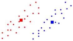
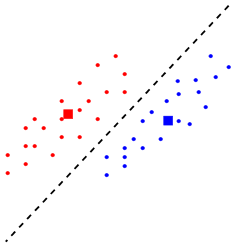
Example:
Suppose we have the following data where d=2 and
n=2. The classes are shown in red and blue. The mean points are
shown as square bullets.
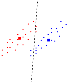
If we apply our simple rule then the boundary
between the two classes is just the perpendicular bisector
joining the two means.
Do you think that it is a good classification boundary? Isn't the
following boundary better?
The second boundary took the "shape" of the classes in
account. To see how we may capture the same idea mathematically
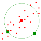
consider just the red cluster:
We have shown two new items (in green) that are equidistant from
the class mean (according to usual Euclidean distance). But will
you be eqaully happy to consider these two items as belonging to
the red class? No, right hand point is actually quite far from
the class, while the left one is well inside the class. This is
because of the unequal spread of the classin the two
directions. So the "conceptual distance" of a point from the
class mean must be scaled down the spread of the class in the
direction connecting the mean to the point. This is the idea
behind Mahalnobis distance. If the mean is at μ and the
new point is at x and the covariance matrix is
Σ then we should consider
(x - μ )' Σ-1 (x-μ) .
So a better method will be to classify the new point as belonging
to the class i that minimises
(x - μi )' Σ-1 ( x -μi ) ,
ie, minimising
x' Σ-1 x - 2μi' Σ-1 x + μi' Σ-1 μi ,
ie, minimising
- 2μi' Σ-1 x + μi' Σ-1 μi .
Thus you put a new measurement vector x in class 1 iff
2(μ2 - μ1)' Σ-1 x < μ2' Σ-1 μ2 - μ1' Σ-1 μ1.
This is just a half space. The boundary is the straight line (or
hyperplane, in general)
2(μ2 - μ1)' Σ-1 x = μ2' Σ-1 μ2 - μ1' Σ-1 μ1.
Well, this is what is called LDA.
◼
Notice that for any given positive definite Σ the
following function
dist( x , y ) = √[ (x-y)' Σ-1 (x-y) ]
is a metric on IRd. If there are c classes then
LDA creates the Voronoi tesselation of this metric space
generated by the class means μ1 , ..., μc. Voronoi
tesselation means a parition where each block consists of all
points that are closer to one μi than the other
μj's.
The following interactive diagram (taken from http://www.cs.cornell.edu/home/chew/Delaunay.html)
will give you a better idea.
Voronoi tesselation generator (click with
your mouse)
The above animation uses Euclidean distance (which corresponds to
Fisher's LDA with Σ = I).
How good is LDA as a classification method? Are the class means good representatives
of clas centres? Is the covariance matrix a good way of capturing
the shape of a class? What if different classes have different
shapes? This method is good if the measurements all have
multivariate Gaussian distribution with same covariance matrix
Σ but different means.
How Fisher originally thought about LDA
Fisher worked with just c=2 classes, but general d.
His original intention was to project everything down to
1-dimension, so that he could clearly visualise the separation
between the two classes. Accordingly he looked for a vector
l such that the
SSB / SSW
criterion of 1-way ANOVA is maximised. The numerator is just the
variance of the (projected) class centres: l' μ1 and
l' μ2. Since variance of two numbers is just a multiple
of their squared difference, this is essentially
( l'μ1 - l'μ2 )2 = l' δ δ' l,
where δ = μ1 - μ2.
The denominator is just
l' Σ l.
Using standard linear algebra the maximum is attained when
l is an eigenvector of Σ-1 δ δ'
corresponding to its largest eigenvalue. But this matrix actually
has rank 1 and its sole nonzero eigenvalue is δ'
Σ-1 δ. An eigenvector corresponding to this
eigenvalue is Σ-1 δ.
Thus Fisher's presciption was to take l = Σ-1 δ,
and to base the classification on l' x where x is
the new measurement vector. This is precisely what we did in the
first approach using Mahalnobis distance.
Fisher's approach has the disadvantage that no obvious
generalisation exists if Σ changes from class to
class, or if c > 2. But the Mahalnobis distance approach
works in those cases also.