Archimedean copula

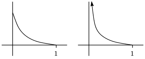
Let φ:(0,1]→ [0,∞) be a strictly decreasing, convex, continuous function with φ(1)=0. Two possible graphs look like:

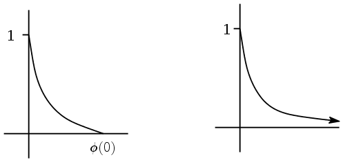
We shall swap the two axes to define a new type of inverse φ^[-1] : [0,∞)→[0,1]. The plots of the inverses of the above two examples look like:

The exact definition is


φ^[-1] (x) = φ^-1 (x) if x ∈ [0,φ(0+))
              = 0           else

Then it is not difficult to see the following results:

φ^[-1] is again continuous and convex. Also it is decreasing (not necessarily strictly).
∀ x∈ (0,1] φ^[-1] (φ(x)) = x.
∀ x∈ [0,∞) φ(φ^[-1] (x)) = min{x,φ(0)}.

Theorem Let φ:(0,1]→ [0,∞) be a strictly decreasing, convex, continuous function with φ(1)=0. Then

C(x,y) = φ^[-1] (φ(x)+φ(y))

is a copula.

We shall prove this later. This motivates the following definition:

Definition Let φ:(0,1]→ [0,∞) be a strictly decreasing, convex, continuous function with φ(1)=0. Then

C(x,y) = φ^[-1] (φ(x)+φ(y))

is called the Archimedean copula generated by φ.

Note that if α>0 is any constant and φ(·) is as above, then φ(·) generate the same copula.

A sort of converse to the above theorem is also true, though of not much use in statistics:

Theorem Let φ:(0,1]→ [0,∞) be a strictly decreasing, continuous function with φ(1)=0 such that

C(x,y) = φ^[-1] (φ(x)+φ(y))

is a copula.

Then φ must be convex.

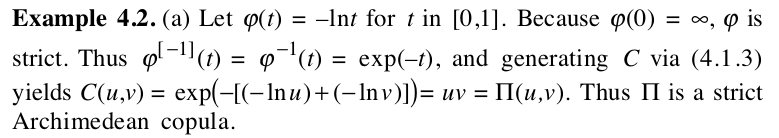
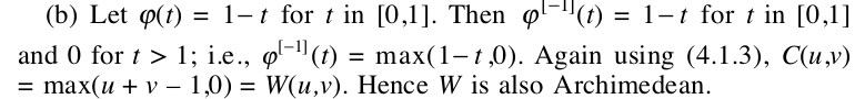
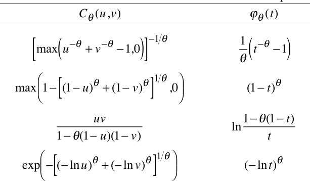
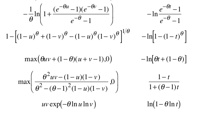
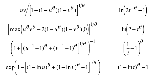
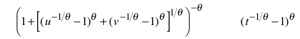
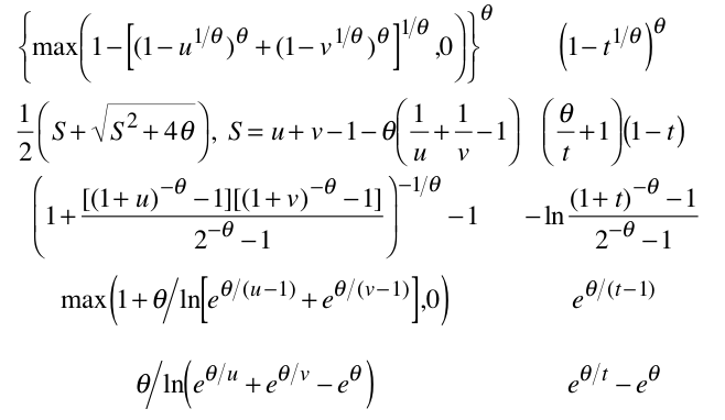
Choosing φ appropariately gives rise to many useful Archimedean copula. Here are a few examples from the book by Nelsen:

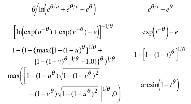
In univariate set up we are more interested in families of distributions rather than individual distributions. Similarly, in a multivariate set up, we are more interested in families of Archimedean copulas than in single Archimedean copulas. For this we choose a φ with one or more parameters. The following list is from Nelsen:

The approach to multivariate (or rather bivariate) modelling using these families may be summarised as follows:

First we need to familiarise ourselves with the shapes of standard univariate distributions, and standard bivariate copulas. We may consider these as two libraries, one for marginals and one for copulas.
Given a bivariate data set we should draw the marginal histograms and pick suitable families of marginals from the library.
Also we should pick a family of copula from the other library.
The chosen marginal families and copula family define a family of bivariate distribution via Sklar's theorem.
We can now perform parametric inference with this family: estimation, goodness-of-fit, testing etc.

Picking a suitable family of copulas is the trickiest step. We shall later learn techniques to do so.

Some interesting properties of Archimedean copulas

A copula is a function C:[0,1]×[0,1]→[0,1], and hence can be viewed as a binary operation on [0,1]. For an Archimedean copula, this binary operation has interesting properties: it is commutative and associative. Also repeated application of this binary operation on the some x∈ [0,1] results in a sequence

x, C(x,x), C(C(x,x),x), C(C(C(x,x),x),x), ...

If we denote the n-th entry in this sequence by Cⁿ (x) (slightly different notation than used in class), then we have

C¹ (x) = x , C² (x) = C(x,x), C³ (x) = C(C(x,x),x), ...

We can use induction to prove that

Cⁿ (x) = φ^[-1] ( n φ(x) ).

Then it is easy to see the following theorem:

Theorem

∀ x,y∈ [0,1] ∃ n∈ IN Cⁿ (x) > y.

The similarity between this result and the Archimedean property of IR has given rise to the name "Archimedean copula". The theorem itself requires Archimedean property of IR for its proof.

Comment Box is loading comments...