We know that if X is a continuous real-valued random
variable with distribution function F, then F(X) is
a random variable with Unif(0,1)
distribution. Unfortunately, this result fails for discrete
random variables. However, the result has a converse which holds
for all random variables (discrete/continuous):
If U ∼ Unif(0,1) and F is any distribution
function, then X = F- (U) is a random variable with
distribution function F, where F- is the generalised
inverse of F defined as
F-(a) = min { x ∈ IR : F(x) ≥ a }.
These two results make Unif(0,1) a "common meeting point"
among all continuous distributions: Start with any continuous
random variable X with distribution function F,
then apply F to X to arrive at a Unif(0,1)
random variable. Then take any distribution function G,
and compute G-(F(X)) to get a random variable with that
distribution function.
The concept of copula is the multivariate analog
of Unif(0,1). We shall restrict our treatment
to IR2 only. The concept is eqaully applicable to any IRn.
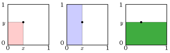
Clearly
C(x,y) must be 0 if x < 0 or y <
0
Also it must be 1 if x,y ≥ 1.
Since we
insist that the marginals are both Unif(0,1), hence
we must have
C(x,y) = x if y≥ 1
and x∈ [0,1)
C(x,y) = y if x≥ 1 and y∈
[0,1)
So the only freedom we have about choosing a copula is
in (0,1)×(0,1). So we shall specify a copula only
on [0,1]×[0,1]
Why care?
Before going into any complicated math, let's convince ourselves
why we should care about copula at all. A short answer is:
The
concept of copula helps us to create many multivariate
distributions with specific properties.
Let's elaborte:
Suppose that we want to model a bivariate data (X,Y),
where X appears to have a Cauchy(θ, 1)
distribution and Y ∼ N(μ, σ2 ) and also they
appear to be quite strongly positively correlated. We would like
to capture this in a model so that we can employ familiar tools
like MLE to estimate the paramters, or test if indeed X,Y
are correlated or not. The problem is to come up with a bivariate
distribution that satisfies all these conditions:
X∼ Cauchy
Y∼ Normal
X,Y are possibly correlated
Here is a simple solution:
Start with (U,V)∼ N2((0,0), (1,1), ρ).
Let W = Φ(U) and Z = Φ(V),
where Φ is the N(0,1) distribution
function.
Now let F be the Cauchy(θ,1) distribution
function. and G be the N(μ,σ2 )
distribution function. Let X = F-1(W) and Y = G-1(Z).
Convince yourself that the joint distribution of (X,Y) has
the desired property. Now let's understand this process step by
step using copula:
We started with any bivariate distribution (with continuous
marginals) having the necessary correlation structure.
Then we "chopped off" the marginals to get (W,Z). The
distribution function (W,Z) is a copula.
Finally, we "attached" marginals of our choice to the copula.
Thus copulas allow us to mix any correlation structure
with any marginals. The term "correlation structure" must not be
construed to mean only product moment corrleation. Here it means
any interrelation among the random variables. Indeed, it is a new
concept, and this is precisely what a copula aims to capture: how
the marginals are coupled inside a joint distribution.
Heading for the theory
Any multivariate distribution is composed of marginals and a
copula. Much of the
theory of copula revolves around this relation:
Multivariate distribution ↔ (copula, marginals)
Sklar's theorem (which may be called the fundamental theorem of
copula) states that (copula, marginals) uniquely determines a multivariate
distribution. The opposite direction is slightly tricky: A multivariate distribution always
uniquely specifies its marginals. If the marginals also happen to
be continuous, then the copula will be unique as well. But if at
least one marginal fails to be continuous, then all that we can
guarantee is the existence of at least one copula, but uniqueness
will fail.
The proof of the first half is trivial: Start with C,
which is already a multivariate distribution function. So there
exists random variables U1,...,Ud with joint
distribution C. Define Xi = Fi- ( Ui ).
Then directly show that the given F is simply the joint
distribution of ( X1 ,..., Xd ).
The proof of the converse part is easy if all the marginals are
continuous: Since F is a multivariate distribution
function, so there are random variables X1,...,Xd with
joint distribution F. Let F1,...,Fd be the
marginals. Define Ui = Fi(Xi). Choose C as the
joint distribution of U1,...,Ud.
If some of the marginals are not continuous, then the proof is
somewhat technical in nature.
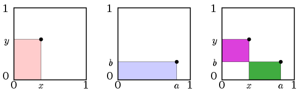
Comparing red and blue, C(x,y)≤ x. Similarly comparing
red and green, C(x,y)≤ y.
So C(x,y)≤ M(x,y).
What is the probability that (X,Y)∈ blue ∪
green?
It is
P(blue) + P(green) - P(blue ∩ green) = P(blue) + P(green) -
P(red) = x + y - C(x,y).
Being a probability it is must be ≤ 1.
Hence C(x,y)≥ x+y-1. And also C(x,y)≥ 0
because it is a probability itself.
So C(x,y)≥ W(x,y).
[Q.E.D]
Are these bounds sharp? Yes, because both M(x,y)
and W(x,y) are copulas.
Proof:
Take any two points (a,b) and (x,y)
in [0,1]× [0,1].
C(x,y) = P((X,Y)∈ red), C(a,b)
= P((X,Y)∈ blue)
So
|C(x,y)-C(a,b)|≤ P(green) + P(purple).
Now P(green) ≤ |a-x| and P(purple) ≤ |b-y|.
So
|C(x,y)-C(a,b)|≤ |a-x|+|b-y|.
[Q.E.D]
Constructing a copula
There are three major ways:
Using Sklar's theorem to extract a copula from a
multivariate distribution
Create a copula from scratch
Transform an existing copula
There is hardly anything to be discussed about the first
approach. So let's focus on the second and third.
Creating a copula from scratch
Example:
The product copula is defined as C(x,y)=xy. Of
course, as always, we are specifying the formula only for x,y∈[0,1].
◼
Example:
The minimum copula is M(x,y)=min{x,y}.
◼
Example:
The function W(x,y)=max{x+y-1,0} is a copula.
◼
Transform an existing copula
Here we start with a copula and obtain (X,Y) from it. Then
we take any (measurable) function f:[0,1]2 →
[0,1]2 such that the marginals of f(X,Y) are
again Unif(0,1). Then the distribution function
of f(X,Y) is a copula.
It may not be readily obvious how to get such transforms. One way
is to use a shuffle. Here we split [0,1] into k
equal subintervals, and permute them.