For a normal model (homoscedastic/heteroscedastic) the R functions lda and qda
that we had used earlier can perform Bayesian classification as
well. Let's apply this on our
familiar banknote dataset.
x = read.table('banknote1.txt',head=T)
names(x)
This
is the same data set , but the last column is given as strings
("genuine" and "forged" instead of numbers). This can be seen
from the output of the following command.
x [ c(1:3,101:103) , ]
Now we want to invoke the lda function from
the MASS library. So we load it.
library(MASS)
Next we have to specify the prior. Suppose that we want to assign
prior probability 0.1 to "forged" and 0.9 to
"genuine" (ie, we believe that 10% of all banknotes of
this particular denomination are forged). So the prior is a
vector with two components, 0.1 and 0.9. The
question is should we write c(0.1,0.9)
or c(0.9,0.1). For this need to know which come
first inside R: "genuine" or "forged"? The answer is to make a
frequency distribution of this variable:
with(x, table(Y))
The output shows that, inside R, "forged" comes before
"genuine". So we should use the prior c(0.1,0.9).
So the lda function may be called like this:
with(dat, plot(X , Y ,
               col = class , pch=20 , cex=2))
points(400,80,pch='x',cex=2,col='magenta') #A new point to be classified
R chooses the colours for us. This is cool, but it is difficult
to understand which colour is for which class. So it is usually
better to assign our own colours:
mycol = c('red','green','blue')
with(dat, plot(X,Y,col=mycol[class],pch=20,cex=2))
points(400,80,pch='x',cex=2,col='magenta') #A new point to be classified
Now we shall apply C&RT. First we show the simplest usage:
library(rpart)
tr=rpart(as.factor(class) ~ X + Y, data=dat)
If you try to print the tree tr like
tr
the output looks pretty confusing:
A more legible output may be obtained by plotting it as a tree:
plot(tr)
text(tr)
Depending on your system, some of the labels may be clipped
off. Then you need to set your margins appropriately:
Don't forget to restore the margins to their original value
before plotting something else.
par(oldpar)
Let's predict the class of the new case:
predict(tr, list(X=400,Y=80))
A closer look
We talked about the GROW and PRUNE stages of C&RT. What you saw
just now is the outcome of the GROW step. R will never prune a
tree until you tell it to do so.
For our toy problem we had listed all the subtrees in the last
class and had computed
fα (T) = R(T) + α |T|
for each. These we linear functions of α. We shall
now plot them using R.
If you are saving this in a file, then don't forget to uncomment
the following line.
#dev.off()
So we see that α = 35/4 is the value
of α at the knee. We obtained this by brute
force. Now let us see how we can get the same info from R. Invoke
the rpart function again, but now with the
additional control parameter that asks R to explore
all values of α>0. The name cp is what R
uses to mean the minimum permissible value of α.
tr=rpart(as.factor(class) ~ X + Y, data=dat,
         control=rpart.control(cp=0))
Now let's find the "knee" (or "knee"'s in a more general problem):
printcp(tr)
Look at the CP column. It has two entries: 0.25 and 0.00. It
means that there are two "critical" values for α, the
first is 0.00, which is the minimum value, and second is the
"knee" we were looking for. But we know that the knee should be
at α = 35/4. Why is it reported as 0.25 then?
This is an idiosyncrasy of R: it divides all the columns
(except nsplit) by the number of misclassifications
at the root node, which is 35 in our
example. Thus α values are 0 and 35×
0.25 = 35/4 as we expected.
The nsplit column tells us the number of splits in
the best tree starting from that value
of α. Thus, 4 corresponds to the full tree,
and 0 corresponds to just the root node.
The rel error gives the resubstitution errors (of
course scaled down by 35, hence called "relative"
error). We shall discuss the other two columns soon. But before
that let us see how to prune the tree:
tr1 = prune(tr,cp=0.3)
plot(tr1) #Oops!
Of course, here the pruned tree is just the root node, so R
refuses to plot it!
Here we get a very simple tree! Just compare this with the LDA
classifier. Indeed, one important reason behind th popularity of
C&RT is the simplicity and easy interpretability of the
classifers it produces.
In both our examples the trees turned out to be hopelessly
simple, allowing us no chance to prune the tree in a nontrivial
fashion. The next example (taken from the vignette of
the rpart package) is more nontrivial.
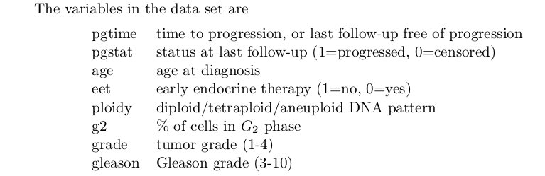
Prostage cancer data
The data set comes with the rpart package. Load it
using
data(stagec)
Or you may download it here, put it
in your working directory and load it with
load('stagec.rda') #Creates a new variable stagec
names(stagec)
We know how to interpret the first three columns. Remember that
here the scaling factor is 54, the number of
misclassifications in the root node. Now we shall learn about the
last two columns. In order to find the best
value of α R automatically performs 10-fold
CV for each of the 6 best subtrees corresponding to
the α values in the intervals between the
"knee"s. Here is how it proceeds:
For each such interval
   R picks a represenative value of α.
   Then R splits the data randomly into 10 parts.
   For each of 10 parts
     R applies C&RT to GROW a tree using the data minus that part.
     R applies the chosen value of α to PRUNE the tree.
     R uses this tree to predict the left out part.
     R records the number of misclassifications made.
   End for
   Now R has 10 misclassifications one for each part.
   These are averaged and average is called xerror.
   The std error of this xerror is called xstd.
End for
For each interval we thus have one xerror and one xstd.
These are what you see in the last column. The idea is to choose
the interval giving the least xerror. However, CV involves
randomisation, and so minor differences in xerror values may be
attributed to chance. That's where xstd comes into picture. A
rule of thumb is to consider the minimum xerror, and to consider
any xerror falling as "basically the same as" the minimum. Choose
the largest α value among these
(largest α means smallest tree). This procedure is
simplied by the plotcp function: