Date: Jan 29, 2014
[[Update:[Wed Jan 31 IST 2018]]
A more formal look at cross-validation
We have
already seen that CV is a way to assess the performance of a
supervised classification method. Given a supervised data set
and a supervised classification method, it produces a number that
measures how badly the method performs. Here it is important to
distinguish between a supervised classification method and the
classifier it produces. For example Fisher's LDA is a supervised
classification method. For a particular data set it may produce a classifier like
"Put a case in class 1 if 2.353 X1-4.867 X2 < 3.509."
This is a classifier. We can think of LDA as a function of the
data. This particular classifier is the value produced by this
function for a particular data set. Thus for a supervised data set Train, we
have a classifier LDA( Train ) obtained by LDA to it. Now given another data set
Data2
we can assess the performance of LDA( Train ) on Test. Suppose we do this by
the proportion of wrong classifications:
Loss ( LDA ( Train ) , Test ) .
If we reuse Train to serve as Test then we get
Loss ( LDA ( Train ) , Train ) .
This is called resubstitution error, and is generally an under-estimate of the
true error rate. Judging a classification method based on the resubstitution error usually leads to
overfitting. Cross-validation is one attempt to counter this. Here we randomly split
the supervised data into k parts (typically k=5 or 10 leading to
5-fold or 10-fold CV):
Data1 , ... , Datak .
Each part should represent the entire data set. Thus simple
random sampking of cases is usually not a good idea. Now the CV error rate is defined as
mean of Loss ( LDA ( Data-i ) , Datai ) , i=1 , ... , k.
It must be bourne in mind that CV is often not enough to remove overfitting.
Bayesian Classification
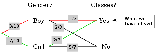
In elementary probability classes we solve problems like the following.
A class consists of 3 boys and 7 girls. Among the 3 boys only 1 wears glasses. Among the 7
girls there are exactly 2 with glasses. A student is selected at random. If the selected student
wears glasses, what is the chance that the student is a boy?
Such a problem requires Bayes' Theorem, and the computation may be elegantly presented in the
form of a diagram:
Bayes diagram
There are two paths (red and green) to the what we have observed. Their probabilities are
Given that we hae taken one of these paths, we want to know the conditional probability that we have taken
the red path:
P(red) / [ P(red) + P(green) ].
Think of this as a classification problem. The students are the cases to be classified into two classes
Boy and Girl. We have only one measurement "Does the student wear glasses?". We can compute
the posterior probabilities of the student being a boy and being a girl. Then classifiy
the student in the clss with the higher posterior. In fact, the posteriors also reflect
how confident in our decision.
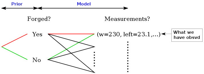
In the banknote example
we can have a similar (infinite) diagram:
Bayes diagram
Here also we can proceed in a similar way.
This approach has one advantage: it can incorporate losses. To understand this consider a real life
example of credit risk analysis. Before giving loan to an applicant a bank has to assess his
credit-worthiness, ie, whether he is going to default or not. For this the bank makes lots of
measurements about the applicant (monthly income, credit history, number of bank accounts, age, etc).
Based on these measurements the appicant has to be classified into one of two classes: Good or Bad.
The bank will use its own past records to get a supervised data. Suppose that the bank has data about
10000 past cases where the loan was granted. Is it reasonable to assume that about half of these were Good
the rest being Bad? No, then the bank would have been bankrupt by now! Only a very small number (say 50) of
these cases will be Bad. If you apply any of the classifiers we have learned about, they will
all suggest classifying every future case as Good, thinking that Bad is a rare event (with probability
0.005), and hence may be ignored. But that is not the right thing to be done. Those 50 cases
are in fact the most important cases. They are the cases that has defeated the bank's already
efficient fraud detection scheme. So if we want to improve the detection we must not ignore these! It
is here that the concept of a loss function arises:
L ( verdict | truth ).
This measures the amount of loss incurred when you make a mistake. For example, we may take
L ( Bad | Good ) = 1,
L ( Good | Bad ) = 100,
which makes giving loan to a Bad guy a much more serious mistake than refusing loan to a Good guy.
We of course define
L ( Bad | Bad ) = 0, L ( Good | Good ) = 0.
Now instad of choosing the class with higher posterior probability we compute the posterior risk, which
is another term for the expectation of the loss function under the posterior distribution. Let us
take the example of students to illustrate. Suppose we have the loss function
L ( Boy | Girl ) = 1,
L ( Girl | Boy ) = 10,
L ( Girl | Girl ) = 0,
L ( Boy | Boy ) = 0.
Thus here mistaking a Boy for a Girl is a 10 times more serious mistake than the opposite mistake.
As before we select a student at random and find that s/he wears glasses. We have two possible
decisions: Boy and Girl. Let's compute the posterior risk for each. We had already computed
the posterior probabilities:
P (Boy | Glasses ) = 1/3 and P ( Girl | Glasses ) = 2/3.
If we give the verdict "Boy", then the posterior risk is
L( Boy | Boy ) P( Boy | Glasses ) + L( Boy | Girl ) P( Girl | Glasses ) = 2/3.
Similarly, the posterior risk for the verdict "Girl" is
We see that the posterior risk is lower in the first case. So we give the verdict "Boy".
Caveat
Bayes classification, as well as other Bayesian methods, suffers from a serious drawback. One has
to supply reasonable prior probabilities, and (optionally) a loss function. Though prior probabilities and
loss functions are present in all problems in principle, they are usually very hard to quantify.
The outcome of a Bayesian method is very sensitive wrt the choices of prior and loss functions, ie, even
seemingly minor changes in these may drastically change the conclusion.
This very drawback, however, makes Bayesian methods popular among dishonest practitioners of statistics.
They use their own intuition and subjective judgements to draw a conclusion, and then back calculate
priors and loss functions that would lead to those conclusions. Then they can pass off their
dubious subjective judgements as objective findings supported by Bayesian computation. In this sense,
Bayesian statistics often plays the role of computer horoscope, a scientific varnish on unscientific
practices.
Classification and Regression Tree (C&RT)
Today we shall learn about a very versatile and popular
supervised classification technique called C&RT. Unlike LDA and
QDA it is a nonparametric method. We shall start with an example.
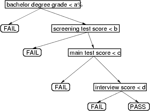
Example:
Consider students seeking admission to ISI. The record for each
student consists of 4 explanatory variables: Bachelor's degree
grade, screening test score, main test score, interview score.
Based on these we decide whether a student should be admitted or
not (PASS or FAIL). As we all know the decision process used at
ISI may be expressed as a tree.
ISI
admission tree
This is called a (binary) classification
tree. It puts each student in a class: PASS or FAIL. Each leaf
node is labelled with a class name ("PASS" or "FAIL"). Each inner
node is labelled with an inequality of the form
Xi < some number,
where Xi is one of the
explanatory variables. If the inequality holds for a student we
follow the left branch, else we follow the right branch.
◼
Each branch in the tree partitions the sample space.
The following interactive animation will help to clarify the
idea. Suppose we have c=3 classes and d=2
measurements. A typical scatterplot (with colour-coded classes)
is shown in the pink box below. We shall keep on splitting the
box with horizontal and vertical lines until each block is "pure"
(ie, contains points of only one colour). This can be done in
many ways. One way will be demonstrated if you repeatedly click
the "Click" button.
Carefully notice how the binary tree to the left corresponds to
the partitioning. Each leaf node corresponds to one block of the
partition.
Misclassification rate
Suppose someone gives us a classification tree as above (with
a,b,c,d replaced by actual numbers.) Based on a dataset how do we
assess its performance? One way is to apply the tree to each
case in the data and see what class it is assigned to by
the tree. Since the dataset also tells us the true class for each case,
we can check if the tree has made a mistake.
Do this for all the cases and count the
number (m, say) of mitakes.
mistake. This is the number of misclassifications. Divide it by the total sample size to get the
misclassification rate.
Using C&RTα
While we prefer trees with a low number misclassifications, we
also want our tree to as small as possible. Large trees require
us to find many cut-off points and usually tend to overfit the
data. There is a trade-off between the size of a tree and its
misclassification proportion. Larger the tree less is the
misclassification, but too large a tree will produce overfit.
C&RT is a family of modelling strategies to achieve a balance
between size and misclassification proportion. Each member in the
family is specified by a nonnegative index, alpha (also called a
tuning parameter. It is just a fancy term, and has nothing to do
with the parameters of a model.) We shall call the modelling
strategy for a given value of α as C&RTα . Thus C&RTα
produces a tree that minimises
number of misclassifications + α × #Leaf
For the ISI admission tree, for instance, #Leaf = 5.
The tuning parameter tries to penalise large trees. If α is
large then C&RTα is more likely to produce smaller trees.
It may not be obvious how to choose α. We shall later see how CV
is used to choose a good value for α. But first let us
learn how C&RTα works if some α>0 is given to us.
How C&RTα works
Suppose we are given a training sample of size n. Each record in the data
is a d+1-tuple (X1 , ..., Xd , C). Here the X's are the
measurements and C is the true class. The idea is that in future we
shall have more cases for which only the X's will be known. Then we shall
use our tree to predict their classes.
C&RTα effectively finds a good way to partition the
space recursively, so that each block is as homogeneous as possible.
This is done through two steps:
GROW
PRUNE
GROW
For d=2, the first split is either a horizontal or a vertical line through the
entire sample
space. So we have two things to determine in the first split: orientation
(ie, horizontal/vertical) and where to draw the line.
Notice that due to the discrete nature of the data points it is enough to
consider only finitely many lines of either orientation. This is because,
until a line
crosses a sample point the misclassification proportion remains
unchanged.
In general there are n lines to consider along each of the d axes. For
each of these nd lines, we compute the number of misclassifications. This
is done as follows. Label each side of a line with a class using majority vote.
Now count the number of points on either side whose classes
does not match the assigned classes. Add the two numbers.
Choose a line with the minimum number of misclassifications. Resolve
ties arbitrarily.
Now the sample space has been partitioned into two blocks. Each
block has been labeled with a classname (eg, "PASS" or
"FAIL" in the ISI example.) This partition corresponds to
a tree with two leaf nodes and one inner node (the root).
Each leaf node is labelled
with a classname. The inner node is not labelled with an inequality. Note that the
leaf nodes correspond to the blocks of the partition.
Carry out
the above procedure separately for each of the blocks.
Thus each of these blocks
will produce two blocks and so on.
The next question now is: "When to stop?"
The answer is: Do not split a block further if
either
the number of sample points in it is less than 5,
or
the block is homogeneous, ie all the points in it belongs to
the same
class.
The number 5 of course has no magic associated with it. You may choose
any other threshold to decide when a block has too few points to warrant
further
partitioning. In fact, if you make this threshold equal to 1, all the
blocks would be homogeneous (because any block with just one point is
trivially homogeneous!)
At the end of GROW you are left with a tree that is usually pretty
huge. Each leaf node (ie, each block of the partition) is either
homogeneous or has too few points in it.
PRUNE
The tree obtained by GROW usually overfits the data. So we need to prune
it. It is here that α makes its appearance. We want a
tree that is not too large, and yet fits the data well. So we try
to obtain a subtree T that minimimises
fα (T) = R(T) + α #Leaves(T) ,
where R(T) is the total number of misclassifications produced by
T.
It is instructive to find this minimiser (which depends on
α) by listing all the subtrees in our toy example. Of
course, this approach is prohibitively time consuming for a
practical problem. The following slideshow does precisely this.
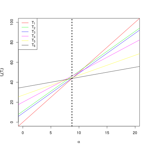
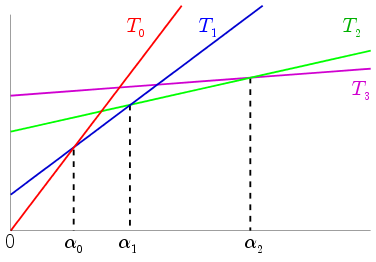
Thus we end up with the following linear functions in α:
For any given α>0 we have to choose a Ti for
which fα ( Ti ) is the minimum. The following plot will
help here.
A close look at the plot shows that T1 is the optimal
tree for α∈ ( 0 , α0 ] where α0
is shown using the thick dashed line. For a>α0 the
best tree is T6, which is just the root node!
Of course, most real life examples are not as drastic as this. In
general we get a finite sequence of values for α:
0 < α0 < α1 < ... < αk ,
for some k ∈ IN, and a corresponding sequence of
nested subtrees of the initial huge tree:
where T0 is the full tree, and Tk+1 is just the root node. For example, a typical case with k=2 is shown below.
For any value of α ∈
[0, α0 ) the best tree is T0. For α ∈
[ α0, α1 ) the best tree is T1, and so
on. The final tree Tk+1 is optimal when α ∈ [
αk , ∞ ) .
As the total number of subtrees of the full tree is huge, finding
this optimal sequence cannot be done by brute force
search. Breiman et al devised a clever algorithm for
this. This is the famous C&RT algorithm presented in their book with the same name.
We shall not go into the details of the algorithm here, but simply treat is a
blackbox that takes a supervised data set and an α>0 as its input, and produces
a classification tree as its output. Think of this as a function
C&RTα (data) = α-optimal classification tree.
The next question is: how to choose α ?
The answer is: Cross-validation.
Cross-validation
We have already seen that CV is a way to assess the performance of a supervised classification method.
Given a supervised data set and a supervised classification method, it produces a number that measures
how badly the method performs. Here it is important to distinguish between a supervised classification
method and the classifier it produces. Each particular tree produced by C&RT is a classifier, while
for each given α , C&RTα is a classification method.
CV is a way to assess the performance of a classification method, not
that of a classifier.
Choosing a good value of α may be considered as choosing a good classification method
among the set
{ C&RTα : α > 0 }.
For this purpose we can take a grid of values for α and assess each using CV, and choose the
one that produces the least CV error rate.