$
\newcommand{\v}{\vec}
\newcommand{\col}{{\mathcal C}}
\newcommand{\vb}[1]{\vec{\bar{#1}}}
\newcommand{\bc}{\because}
\newcommand{\ip}[1]{\langle #1 \rangle}$
Applications
Here we shall briefly touch upon various applications of linear
algebra that you will encounter during the B.Stat course.
Let $f:{\mathbb R}\rightarrow{\mathbb R}$ be a differentiable function. Then its
derivative $f'(x)$ is another function from ${\mathbb R}$
to ${\mathbb R}.$ From this once may naively expect that the higher
dimensional analogs of these concepts would be such that the
"derivative" of a "differentiable" function from ${\mathbb R}^n$ to ${\mathbb R}^m$ would be
another function from ${\mathbb R}^n$ to ${\mathbb R}^m.$
Unfortunately, that is not the case. The actual generalisation,
though quite intuitive, is somewhat indirect, and uses linear transformations.
Why do we care about differentiability? Because, certain curves
may be nicely
approximated by a straight line locally, while certain other
curves may not. When we say $f(x)$ has derivative $5$
at $x=1$ we mean that for $x\approx 1$
$$
f(x)-f(1) \approx 5(x-1).
$$
This is made rigorous as
$$
\lim_{x\rightarrow 1}\frac{|f(x)-f(1)-5(x-1)|}{|x-1|} = 0.
$$
This may look different from the familiar definition of
differentiation, but it is the same thing.
Well, "multiplication by 5" is a linear transformation. So the
intuitive way to define differentiability of a
function $F:{\mathbb R}^n\rightarrow{\mathbb R}^m$ at a point $\v p\in{\mathbb R}^n$ is
that for $\v x\approx\v p$ we should have
$$
F(\v x)-F(\v p) \approx D(\v x-\v p),
$$
for some linear transformation $D:{\mathbb R}^n\rightarrow{\mathbb R}^m.$
Of course, this may be made rigorous much as in the 1-dim case,
except that we use norm instead of absolute value:
$$
\lim_{\v x\rightarrow \v p}\frac{\|F(\v x)-F(\v p)-D(\v x-\v p)\|}{\|\v x-\v p\|} = 0.
$$
Careful here: the norm in the numerator is Euclidean norm
in ${\mathbb R}^m$ while the denominator is the Euclidean norm in ${\mathbb R}^n.$
Thus the analog of the "derivative at a point" is a linear
transformation! So if $F:{\mathbb R}^n\rightarrow{\mathbb R}^m$ is differentiable
everywhere then the "derivative" is a function from ${\mathbb R}^n$
to the sapce of all linear transformations
from ${\mathbb R}^n\rightarrow{\mathbb R}^m$!
It is
cuustomary to express a linear transformation from ${\mathbb R}^n$
to ${\mathbb R}^m$ by an $m\times n$ matrix w.r.t. the
Euclidean bases of ${\mathbb R}^n$ and ${\mathbb R}^m.$ If you do that
it will be seen that the matrix representation of $D$ is
just what we call the Jacobian matrix with $(i,j)$-th entry
$$
\frac{\partial F_i}{\partial x_j}.
$$
So it is not uncommon to refer to this matrix (instead of
the linear transformation $D$) as the
derivative. If you do so, something funny happens. It is quite
possible that the "derivative" exists even though $F(\v
x)$ is not differentiable! The function $F:{\mathbb R}^2\rightarrow{\mathbb R}$
defined by
$$
F(x,y) = \left\{\begin{array}{ll}1 &\text{if }x=0\mbox{ or } y=0\\\mbox{any damn formula} &\text{otherwise.}\end{array}\right.
$$
is one such example. Just visualise the function as a surface,
and mentally compute the Jacobian at $(0,0)$ to see what I
mean.
However, if you (correctly) stick to defining the derivative as the linear
transformation (not just a matrix), then no such funny thing happens.
We are all familiar with the chain rule: if $f(x) = g(h(x))$
then
$$
f'(1) = g'(h(1)) \times h'(1).
$$
You may guess its generalisation for higher
dimensions. If $H:{\mathbb R}^n\rightarrow{\mathbb R}^m$ and $G:{\mathbb R}^m\rightarrow{\mathbb R}^k$
and $F = G\circ H,$ then for a point $\v x\in{\mathbb R}^m$ we
have
$$
D_{F,\v x} = D_{G,H(\v x)} \circ D_{H,\v x}.
$$
Here $D_{F,\v x}$ means the linear transformation that the
denotes the derivative of $F$ at $\v x.$
Of course, you represent all the derivatives using the Jacobian
matrices, then you get matrix multiplication:
$$
J_{F,\v x} = J_{G,H(\v x)} J_{H,\v x}.
$$
It is instructive to check that the sizes of the matrices allow
you to perform the multiplication.
The first derivative of a function ${\mathbb R}^n$ to ${\mathbb R}^m$
turned out to be a linear transformation, the second derivative
of a function from ${\mathbb R}^n$ to ${\mathbb R}$ turns out to be a
quadratic form (represented by a real symmetric matrix called the
Hessian).
To understand this consider a smooth function $f:{\mathbb R}\rightarrow{\mathbb R}.$
Take any $a\in{\mathbb R}.$ Then near $a$ the function may be
well-approximated by its tangent: $y=f(a)+f'(a)(x-a).$
Of course, $f(x)$ need not be exactly equal to this
if $x\neq a.$, since $f(x)$ may have a curvature, while
the tangent (being of the form $y=c + m x$) is just
straight. If we allow a quadartic approximation, then we hope to
come closer to $f(x).$ A good approximation is
$$
y = f(a)+f'(a)(x-a) + \frac{f''(a)}{2}(x-a)^2.
$$
A similar thing happens even if $f:{\mathbb R}^n\rightarrow{\mathbb R}.$ Then
the role of $f'(\v a)$ is played by the Jacobian matrix
(which is $1\times n$). In this context (ie, when the domain
is ${\mathbb R}^n$ and codomain is ${\mathbb R}$) the Jacobian has
another name: the grad and denoted by $\nabla f(\v
a).$ Thus
$$
\nabla f(\v a) = \left[\begin{array}{ccccccccccc}
\frac{\partial f}{\partial x_1} & \frac{\partial f}{\partial x_2} &
\cdots & \frac{\partial f}{\partial x_n}.
\end{array}\right]
$$
In this case the quadratic approximation is
$$
y = f(\v a) + \nabla f(\v a) (\v x-\v a) + \frac12 (\v x-\v
a)' H (\v x-\v a),
$$
where $H$ is the $n\times n$ Hessian matrix
with $(i,j)$-th entry
$$
\frac{\partial^2 f}{\partial x_i\partial x_j}.
$$
Under moderate restriction on $f$ (which we assume) $H$
is a symmetric matrix.
When we are trying to find max/min of $f(\v x)$ we naturally
equate $\nabla f(\v a)$ to $0.$ All the values of $\v
a$ where this holds are the candidate points where max/min may
occur.
At any such $\v a$ we have
$$
f(\v x) - f(\v a) \approx \frac12 (\v x-\v
a)' H (\v x-\v a),
$$
which is a quadratic form in $(\v x-\v a).$ Think of $f(\v
x)$ as equal to this quadratic form over some neighbourhood of
$\v a$ in ${\mathbb R}^n.$ Then it is not
difficult to see that
$f$ has a strict local min at $\v a$ if $H$ is PD.
$f$ has a strict local max at $\v a$ if $H$ is PD.
We are all familiar with the integration by substitution for
function from ${\mathbb R}$ to ${\mathbb R}.$ If we substitute $x = u(t)$, then
$$
\int_a^b f(x) dx = \int_{u ^{-1} (a)}^{u ^{-1} (b)} f(u(t)) u'(t) dt.
$$
While we have been using this since our high school days, we are
not often aware that for this $u$ needs to be a bijection
(else $u ^{-1} $ would not make sense). Also it needs to be
differentiable.
If we give $u
^{-1} $ a name, say $v.$ Then the result is
$$
\int_a^b f(x) dx = \int_{v (a)}^{v (b)} f(v ^{-1}(t)) \frac{dv ^{-1}(t)}{dt} dt.
$$
In this form it is more commonly called the change-of-variable
formula.
Here the new variable is expressed as a function of the
existing variable $t = v(x).$ This function needs to be a
bijection (else $v ^{-1} $ cannot be defined), and the
inverse needs to be differentiable.
The multi-dimensional generalisation of this formula is remarkably
similar, except for a strange occurence of determinant:
Suppose that we are integrating $f:{\mathbb R}^n\rightarrow {\mathbb R}$ over
some $S\subseteq{\mathbb R}^n,$ ie, we are computing
$$
\int_S f(\v x) d\v x.
$$
That single integral sign now represents
an $n$-dimensional integration. We are also given a
function $v:{\mathbb R}^n\rightarrow{\mathbb R}^n$ that transforms $S$
to $v(S)$ and is a bijection between $S$
and $v(S).$ We also assume that $v ^{-1} $ is
differentiable over $v(S).$ Let $J(\v t)$ be the
Jacobian matrix of $v ^{-1} $ computed at some point $\v
t\in v(S).$ Then the change-of-variable formula
becomes
$$
\int_S f(\v x) d\v x = \int_{v(S)} f(v ^{-1} (\v t)) det(J(\v t)) d\v t.
$$
A couple of points are worth noting:
Markov chain is a fancy term for a game of ludo played
with a single counter. There is a board (called the state
space) and the counter moves from a position to another
following a die (or some other randomisation rule). Each position
is called a state. A real ludo has different marks
(arrows, snakes, ladders etc) on the board to guide the
counter's motion (or transition) from state to state. This
role is played by a matrix (called the transition matrix)
in a Markov chain. If there are $n$ states, then it is
an $n\times n$ matrix. If the counter is at state $i$
now, then $(i,j)$-th entry is the
probability that in the next step it will be at state $j.$
If $X_k$ denotes the state of the counter at step $k,$
then the $(i,j)$-th entry of the transition matrix $P$
is
$$
p_{ij} = P(X_{k+1}=j|X_k=i).
$$
We are assuming that this is free of $k$ (ie, the same die
is rolled at each step).
An example will help here.
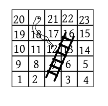
For the following board
Ludo
w2
the state space is $\{1,2,...,23\}.$ Note that the unstable
squares (mouth on snake and bottom of ladder) are not considered
as states. Here the $1$-st row of the transition matrix
contains $\frac16$ in columns $2,3,4,5,6$ and $16.$
The remaining entries in the row are zero.
Notice that $P^2$ is the 2-step transition matrix, ie,
$$
((P^2))_{ij} = P(X_{k+2}=j|X_k=i).
$$
Similarly, $P^k$ is the $k$-step transition matrix.
$X_1$ is the initial position of the counter. Its
distribution depends on the game starting rule. For example, if
the counter always starts at $1,$ then $X_1$ is
degenerate at $1.$ If the counter is kept outside the board,
and enters according to the roll of a fair die, then $P(X_1=i)
= \frac16$ if $i=1,2,3,4,5,16$ and $0$ else.
Whatever, the initial distribution, it can be specified by
a $1\times n$ probability vector. Call it $\v p_1'.$
Note the transpose sign, since it is a row vector. Convince
yourself that the distribution of $X_2$ is
$$
\v p_2' = \v p_1' P.
$$
In general, the distribution of $X_k$ is
$$
\v p_k' = \v p_{k-1}' P.
$$
For many important Markov chains the vector sequence $(\v
p_1,\v p_2,\v p_3,...)$ converges to some probability
vector $\v\pi.$ Then, taking limit of the last equality, we
have
$$
\v \pi' = \v\pi' P.
$$
If only the equation were $P\v\pi=\v\pi,$ we would have
said $\v\pi$ is an eigenvector of $P$ corresponding to
eigenvalue 1. But here have $\v\pi$ to the left
of $P.$ So we say that $\v\pi$ is a left
eigenvector of $P$ corresponding to (left) eigenvalue
1. Of course, we could have also said: $\v\pi$ is an
eigenvector of $P'$ corresponding to eigenvalue 1.
Anyway, we do not need the adjective "left" in front of
eigenvalue, because of the following result.
EXERCISE:Show that for any matrix $A$ the eigenvalues
of $A$ and $A'$ are the same.
However, left eigenvectors are indeed different from the usual
(or right) eigenvectors. We said that the equality
$\v \pi' = \v\pi' P$ results from the fact that
for certain Markov chains the distributions
of $X_k$'s converge. This gives rise to certain mathematical
questions, which are presented in the problems below.
EXERCISE:Show that for any stochastic matrix, $1$ is an
eigenvalue.
EXERCISE:Show that for every stochastic matrix there is a left
eignvector which is a probability vector.
EXERCISE:Show that for a stochastic matrix, all the
eigenvalues $\lambda$ must satisfy $|\lambda|\leq
1.$ Also if $|\lambda|=1,$ then $\lambda=1.$
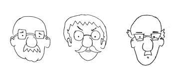
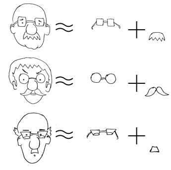
If you want to describe any one of them then there are two ways
to do it:
You can do it like a camera, take a small enough unit,
and then start describing every square unit of area.
This technique is very precise, but generates too much data to
describe a single face.
The second method is to pick a few important features of the
faces (eg, spectacles, moustache), and describe only those
features. Thus
In this technique we do lose some information, but still we are
happy, because we have retained enough information.
To translate this idea to linear algebra, think of each key feature as a long line, eg, one line for
moustache, another for spectacles. Each point along the moustache
line represents one partixular type of moustache. Similarly each
point along the spectacles line denotes a spectacle. In terms of
linear algebra, each key feature is a 1-dim subspace. Each vector
in the moustache subspace is one type of moustache. Similarly,
each vector in the spectacles subspace is a type of spectacles.
PCA is a method to identify these subspaces.
The most desirable property of a key feature is that the
individuals should vary a lot w.r.t. that feature. "The murderer
has one head, two hands and two legs" is not a very useful
description of the criminal, because there is hardly any
variation in the numbers of heads, hands and legs among humans. But
height, hairstyle and fingerprint are very informative, because
there is a lot of variability there. So PCA actually looks for
subspaces along which the data points vary the most.
An example will help here.
The file pca.dat has a data set with 3
columns, X,Y
and $Z.$ The interactive 3D scatterplot is
shown here. Play with it to convince yourself that all the
data points are actually lying almost on a plane. This means that
the data vary in only two directions, not three. If we set up a
new coordinate system with a point in this plane as the origin,
and two vectors along the plane as the $x$-
and $y$-axes, then each point may be expressed as just two
numbers, instead of three.
Here we say that the intrinsic dimension of the data
is $2,$ even though the apparent dimension
is $3.$ The terms "intrinsic" and "apparent" are not
standard, by the way.
There are are many real life data sets where the intrinsic
dimension is substantially smaller than the apparent
dimension. Actually, the intrinsic dimension usually depends on
the complexity of the underlying system, while the apparent
dimension depends on the elaborateness of the measurement. For
example, if we photograph human faces, then the intrinsic
dimension depends on the complexity of human faces, while the
apparent dimension depends on the resolution of the camera.
Given a high dimensional data, we usually want to know the
intrinsic dimension, and are happy if it is much smaller than the
apparent dimension. This is precisely what PCA is useful for.
is a very
popular tool for this.
Suppose we $p$ measurements made on
each of $n$ subects to produce a data
matrix $X_{n\times p},$ where $p$ is large. Let
the $p\times 1$ vector $\v x_i$ denote the measurements
made for the $i$-th subject. PCA looks
for the directions along which the spread of the data is the
maximum. Let a typical direction be given by a unit vector $\v
\ell_{p\times 1}.$ If the covariance matrix of the data
is $S_{p\times p},$ then the amount of spread aong this
direction is given by
$$
\v\ell' S\v \ell.
$$
We know that is maximum iff $\v\ell$ is an eigenvector (say $\v\ell_1$)
corresponding to the largest eigenvalue of $S.$ Then the
direction of second maximum spread is given by a unit
vector $\v\ell$ which is an eigenvector corresponding to the
second largest eigenvalue, and so on. Also the variance of the
data along thoe directions are the corresponding eigenvalues.
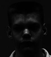
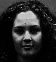
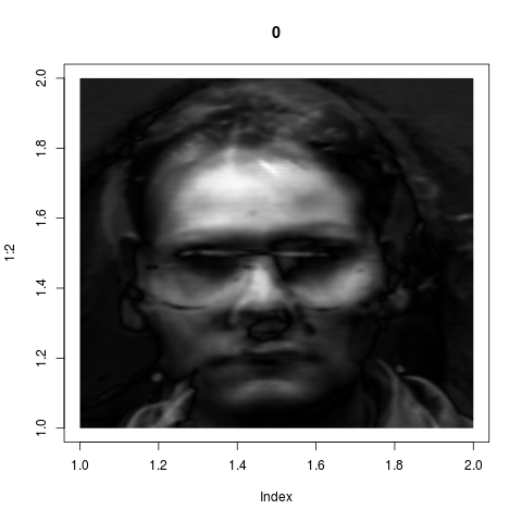
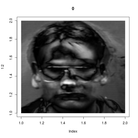
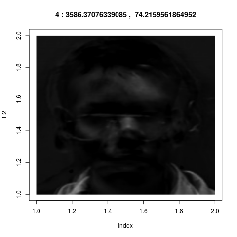
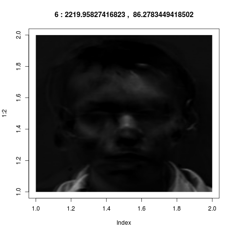
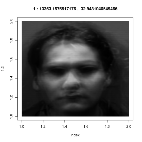
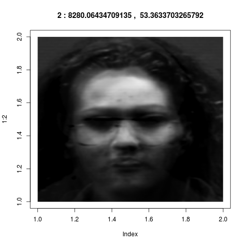
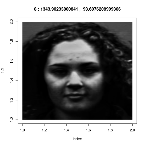
Here is a real life example from image processing.
Faces of 5 men and 5 women are photographed, 5 photos per person. Here are two typical
photos:
Each photo is of size $200\times 180.$ Thus there
are $36,000$ pixels in a single photo, and each pixel
contains a single number (the brightness). So
the $5\times5\times5=125$ photos are like $125$ points
in ${\mathbb R}^{36000}.$ As PCA reveals, these points actually live
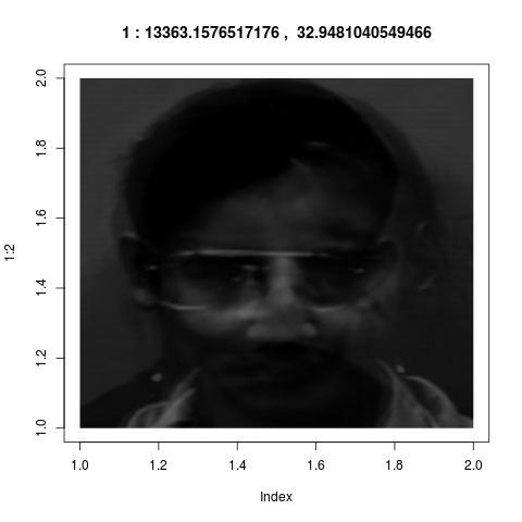
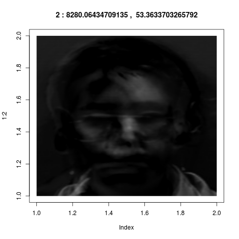
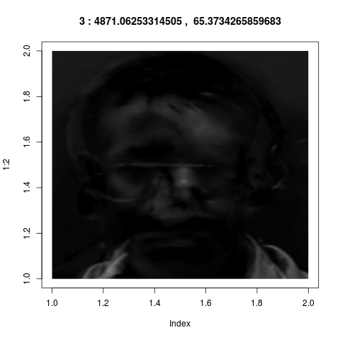
in a $8$-dim subspace (approximately).
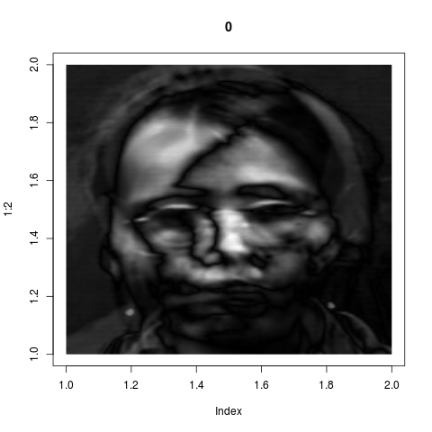
The eigenvectors of $S$ corresponding the 8 largest
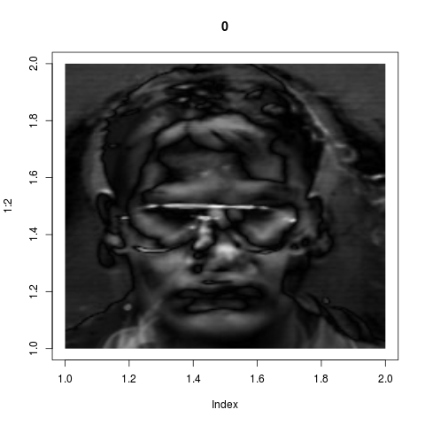
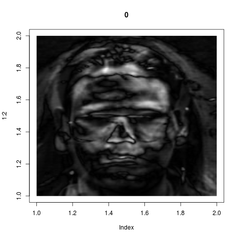
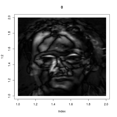
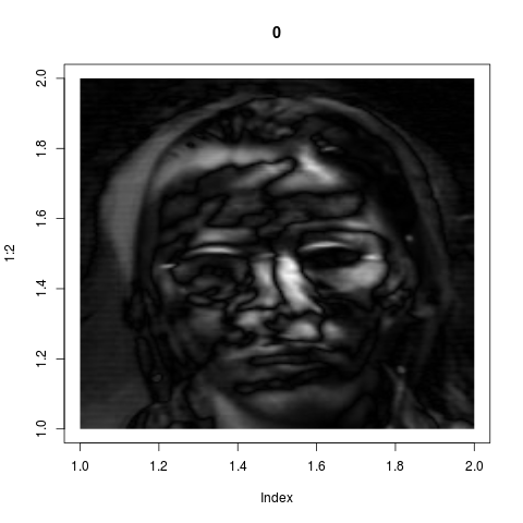
eigenvalues span this subspace. These eigenvectors are the "key
features" as identified by the system. If we wrap back these 8
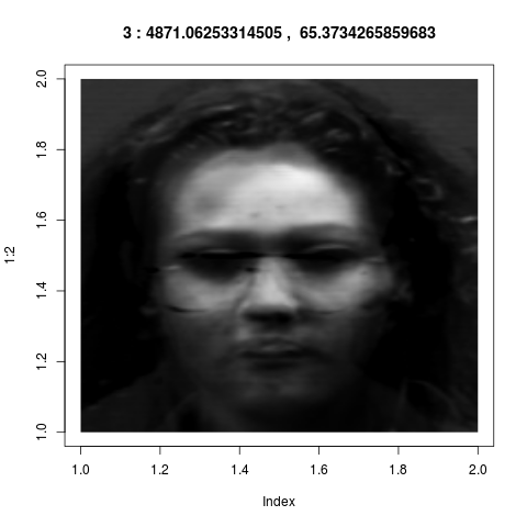
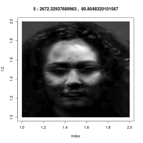
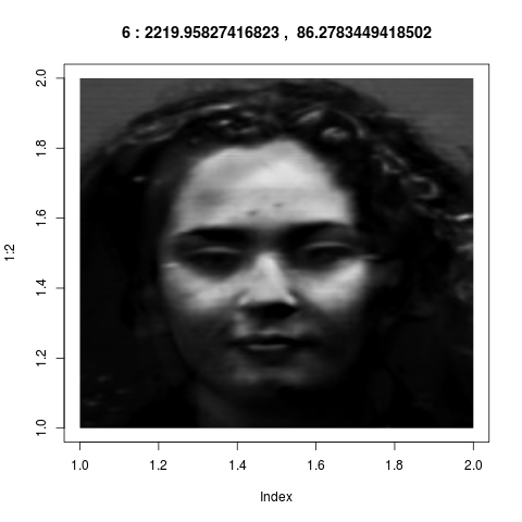
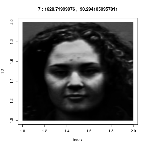
vectors from ${\mathbb R}^{36000}$ into images, they look like
these:
Admittedly these look confusing. They do not correspond to our
intuitive sense of "key features". But if fact, they are much
more powerful than what we could have achieved by intuition
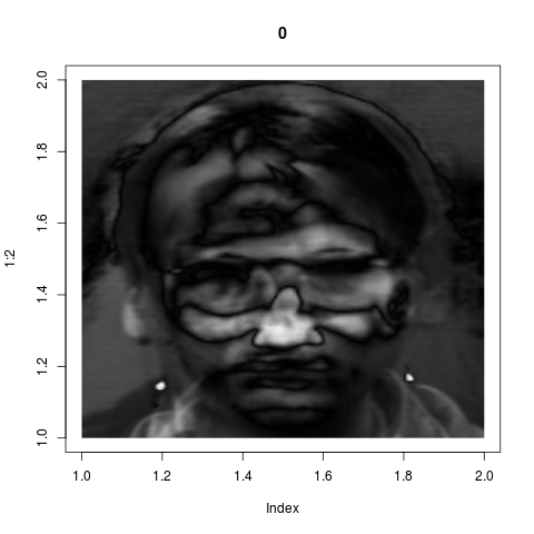
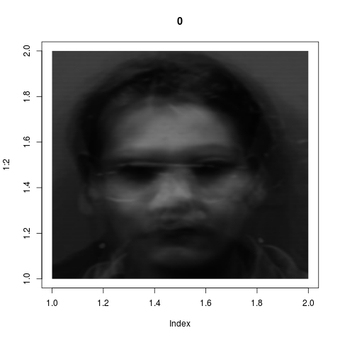
alone. Also here is the mean face:
If we denote this by $\v\mu$ and the $8$ eigenvectors shown
earlier by $\v v_1,...,\v v_8,$ then each of $125$ photos $\v
x$ can be well-approximated by
$$
\v x\approx \v\mu+\alpha_1\v v_i+\cdots+ \alpha_8\v v_8,
$$
Here the coefficients $\alpha_1,...,\alpha_8$ depend on the
particular photo $\v x.$ To give you an idea of the accuracy
of this approximation, we show a sequence of successive
approximations:
$$
\v\mu+\sum_{i=1}^k \alpha_i \v v_i,~~k=0,...,8.
$$
All these data are freely available on the web. Do a google
search for "eigenface" to find these. If you are interested
carrying out the analysis yourself in R, please drop me a line.
The basic steps are:
Load the data as a $125\times 36000$ matrix, each row
being a photo, each column devoted to one pixel position.
Average the rows to get $\v \mu.$
From each column subtract its mean (ie, centre each
column). Call the new matrix $X_{125\times 36000}.$
Since we have already done centering, so the covariance
matrix is simply $X'X,$ which is a huge
matrix $36000\times 36000.$ We want its eigenvalues and
eigenvectors. We know that SVD of $A$ gives eigenvalues and
eigenvectors of $A'A.$ So we just compute SVD of $X.$
If we are given a (possibly inconsistent) system of linear
equations $A\v x = \v b,$ then one way of solving it is via
the least squares method. This means finding a $\v x_0$ such
that $A\v x_0$ is the orthogonal projection of
$\v b$ onto $\col(A).$
The entire course of Linear Models revolves around this idea.
Consider a typical situation where we have some system (treated
as a blackbox) into which a number of inputs are fed, and out of
which a single output is coming out. In all real life situations,
some random issues also enter the system that we cannot eliminate
or detect. So the output is only an approximate function of the
inputs. Many such cases lead to an equation of the form
$$
\v y_{n\times 1} = X_{n\times p}\v \beta_{p\times 1} + \v
\epsilon_{n\times 1}.
$$
Here we have reeated the "apply-inputs-and-see-output"
process $n$ times (possibly with different input
combinations). The output of the $i$-th case is $y_i.$
$\epsilon_i$ is the error input for that
case. The $i$-th row of $X$ is made of the inputs
applied in the $i$-th case. The $\v \beta $ vector are
the unknown coefficients to be estimated that relate the inputs
to the output (and thus is a property of the system).
A typical example could be height-weight relation for men and
women. So the blackbox diagram looks like:
Here height $(h)$ and gender $(g)$ are the inputs
(along with the inevitable random error), and weight $(w)$
is the output. If it is believed that the height-weight relation
is like a striaght line for both genders, and both the straight
lines the slope is the same but the intercept may possibly
differ, then ideally
$$
w = \left\{\begin{array}{ll}a_1 + b w&\text{if }\mbox{ male}\\a_2 + b w&\text{if }\mbox{ female}\\\end{array}\right..
$$
If we have collected height-weight data for 4 men and 3 women,
and have denoted the heights and weights by $(h_i, w_i)$
where $i=1,...,4$ for men and $i=5,6,7$ for the women,
then in matrix notation we have $\v y = X\v \beta + \v
\epsilon,$
where $\v y = (h_1,...,h_7)'$ and $\v \epsilon =
(\epsilon_1,...,\epsilon_7)'.$ Also
$$
X = \left[\begin{array}{ccccccccccc}
1 & 0 & h_1\\
1 & 0 & h_2\\
1 & 0 & h_3\\
1 & 0 & h_4\\
0 & 1 & h_5\\
0 & 1 & h_6\\
0 & 1 & h_7
\end{array}\right]
\mbox{ and }
\v \beta = \left[\begin{array}{ccccccccccc}a_1\\a_2\\b
\end{array}\right].
$$
This is an example of a linear model.
Notice that there are two inputs here (other than the random
error). One input (height) is continuous, while the other
(gender) is discrete. So this linear model is called an ANCOVA
model. If there were no continuous input, then we would have
called it an ANOVA model. If, on the other hand, only continuous
inputs were present, then it would have been a regression
model. But whatever the name, the same concept of orthogonal
projection is used.
The Schur complement of $D$ in $\left[\begin{array}{ccccccccccc}A & B \\ C &
D
\end{array}\right]$ is defined as $A-BD ^{-1} C.$ Of
course, $D$ must be nonsingular for this to make sense.
This has an interesting application in statistics. Suppose that a
sales department collects data on its sales persons. For each
sales person two variables are measured: the age ($X_1$) and
the average amount of daily sale ($X_2$). It is found that
correlation of $X_1$ and $X_2$ is quite high and positive. From this
the sales manager concludes that older sales persons are better,
and hence orders the recruiting department to recruit only
elderly persons.
Is this a wise decision?
No. The high positive correlation between $X_1$
and $X_2$ may not indicate that high $X_1$
causes $X_2$ to shoot up. In fact, it is more likely that
experience with customer handling is main reason behind the
improvement in sale. So the situation is like
more experience $\Rightarrow$ more sale
more experience means more age.
So recruiting fresh elderly persons would not help (since they
have little experience).
But how to statistically validate the effect of experience? We
can measure another variable for each sales person: experience in
years ($X_3$). Then we can take out the effect of $X_3$
from both $X_1$ and $X_2$, and then compute the
correlation between whatever is left of $X_1$ and $X_2.$
One popular way of doing this is as follows.
First orthogonally
project $X_1$ onto $span\{1,X_3\}$
(ie, fit a leat squares straight
line $\hat X_1 = a\cdot 1+ b\cdot X_3$) and then take the
residual vector.
Similarly we extract the component
of $X_2$ orthogonal to $span\{1,X_3\}.$
Now find the correlation between these orthogonal
components. This correlation is called the partial
correlation between $X_1$ and $X_2$
given $X_3.$ We also call $X_3$ the conditioning variable.
In general, there may be many conditioning variables.
It may sound like a rather complicated procedure, but it turns
out that there is a surprising shortcut:
First compute the covariance matrix $\Sigma$ of $(X_3,X_1,X_2).$
Notice the ordering of the variables: the conditioning variables
(here we have just one, $X_3$)
are written first. We assume $\Sigma$ is PD.
Partition $\Sigma$ as
$$
\Sigma = \left[\begin{array}{ccccccccccc}A & B\\B' & C
\end{array}\right],
$$
where $A$ corresponds to the conditioning variables. (Thus,
in our example $A$ is $1\times 1$). Now compute the
Schur complement of $A$ in $\Sigma:$
$$
C - B'A ^{-1} B.
$$
This is a $2\times 2$ matrix, which is again PD. This is
called the partial covariance matrix of $X_1, X_2$
given $X_3.$
Compute the correlation based on this matrix,
(ie, if the entries are $d_{ij},$ then
find $d_{12}/\sqrt{d_{11}d_{22}}$). This number is bound to
be the required partial correlation!
If there are many conditioning variables, then $A$ will be a
large matrix. So computing Schur complement directly may look
daunting. Then there is another shortcut. SImply apply
Gauss-Jordan elimination on $\Sigma$ and do this
until $A$ reduces to $I.$ Then the matrix will look
like
$$
\left[\begin{array}{ccccccccccc}
I & *\\
O & P
\end{array}\right]
$$
This $P$ will be the required Schur complement!
We have learned about different inner products and norms. In
general an inner product over ${\mathbb R}^n$ looks like
$$
\ip{\v x, \v y} = \v x' M \v y,
$$
where $M$ is a PD matrix. Euclidean matrix uses $M=I.$
Here is a situation where $M\neq I$ is a natural choice.
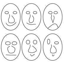
Consider the cartoon faces below:
All the faces are slight variations of each other. There is one
face, however, which is just too much off! Which one?
The last one, of course! No normal human face has two eyes
differing that much. Note the point here: eyes may differ a lot
from face to face, but both the eyes on the same face are
approximately mirror images of each other.
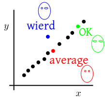
One way to quantify this in terms a norm (induced by an inner
product), is via the Mahalanobis distance. To understand this,
let us focus only on the horozontal lengths of the eyes
(say $X$ for the left eye and $Y$ for the
right). If we collect data on $(X,Y)$ from many faces, then
we expect a scatterplot like this:
Notice that the green dot is further away than the blue dot from
the red dot according to Euclidean norm. But
intuitively, the blue face is much more different from an average
face than the the green one is.
Mahalanobis proposed a new type of norm that coincides with our
intuition. His proposed norm is $\|\v x\|,$ where
$$
\|\v x\|^2 = \v x' \Sigma ^{-1} \v x.
$$
Here $\Sigma$ is the covariance matrix (assumed PD). The
presence of the $\Sigma ^{-1} $ essentially scales down the
data by different amounts in different directions until all the
directions have equal spread, and then computes Euclidean norm
based on the scaled data. It is the multidimensional analog of
stadardisation for 1-dim data: $\frac{x_i - \mu}{\sigma}.$
In statistics we often have to estimate parameter values using a
given data set. The most popular method for doing this is called
maximum likelihood estimation (MLE), which requires us to
maximise a particular function. In a frequently occuring set up
involving the multivariate normal distribution the
result $tr(AB)=tr(BA)$ proves useful as we show now.
At one place in the computation we need to minimise
$$
\sum_{i=1}^n (\v x_i-\v \mu)' \Sigma ^{-1} (\v x_i -\v \mu )
$$
w.r.t. $\v\mu\in{\mathbb R}^k.$ Here $\Sigma_{k\times k} $ is the fixed PD matrix
and $\v x_1,...,\v x_n$ are our data points in ${\mathbb R}^k.$
We proceed as follows.
\begin{eqnarray*}
\sum_{i=1}^n (\v x_i-\v \mu)' \Sigma ^{-1} (\v x_i -\v \mu )
& = & tr(\sum_{i=1}^n (\v x_i-\v \mu)' \Sigma ^{-1} (\v x_i -\v \mu ))~~\left[\mbox{$\bc tr(A_{1\times 1})=A$}\right]\\
& = & \sum_{i=1}^n tr((\v x_i-\v \mu)' \Sigma ^{-1} (\v x_i -\v \mu ))~~\left[\mbox{$\bc tr(A+B)=tr(A)+tr(B)$}\right]\\
& = & \sum_{i=1}^n tr( \Sigma ^{-1} (\v x_i -\v \mu ) (\v x_i-\v \mu)')~~\left[\mbox{$\bc tr(AB)=tr(BA)$}\right]\\
& = & tr( \sum_{i=1}^n \Sigma ^{-1} (\v x_i -\v \mu ) (\v x_i-\v \mu)')\\
& = & tr( \Sigma ^{-1} \sum_{i=1}^n (\v x_i -\v \mu ) (\v x_i-\v \mu)')\\
& = & tr( \Sigma ^{-1} \sum_{i=1}^n (\v x_i -\vb x+\vb x-\v
\mu) (\v x_i-\vb x+\vb x\v \mu)')~~\left[\mbox{where $\vb x = \frac1n\sum\v x_i$}\right]
\\
& = & \cdots\\
& = & tr(\Sigma ^{-1} (A+n (\vb x-\v \mu)(\vb x-\v \mu)')),
\end{eqnarray*}
where $A_{k\times k}$ is free of $\v \mu.$
Thus it is enough to minimise $tr(\Sigma ^{-1} (\vb x-\v
\mu)(\vb x-\v \mu)')),$ which may be written as $tr((\vb x-\v \mu)'\Sigma ^{-1} (\vb x-\v
\mu))) =(\vb x-\v \mu)'\Sigma ^{-1} (\vb x-\v
\mu))), $ since it is a scalar.
Since $\Sigma $ is PD, so is $\Sigma ^{-1}.$ Hence the
minimum value is $0$ attained iff $\v \mu = \vb x.$
In the example above we optimised w.r.t. $\v \mu$
keeping the PD matrix $\Sigma $ fixed. In fact, we need to
optimise w.r.t. $\Sigma $ as well. This eventually leads to
the problem of maximising
$$f(G) = n\log|G|-tr(GA), ~~G \mbox{ is PD}$$
where $A$ is a fixed PD matrix. Remember that the domain
of $f$ is the set of all $k\times k$ PD matrices.
First we decompose $A$ as $A=CC',$ where $C$ is
nonsignular. Then
$$
f(G) = n\log|(C')^{-1} C' G C C ^{-1} |- tr(G C C')
= n\log|(CC')^{-1}|+n\log| C' G C |- tr(C' G C ).
$$
Let $\Delta = C'GC.$ Then (since $C$ is
nonsingular) $\Delta $ takes all possible PD values
when $G$ does so. Hence we can as well carry out the
maximisation w.r.t. $\Delta.$ Then the function is
$$
F(\Delta) = n\log|\Delta| - tr(\Delta).
$$
If the eigenvalues of $\Delta_{k\times k} $
are $\lambda_1,...,\lambda_k,$ then
$$
F(\Delta) = n\sum (\log \lambda_i - \lambda_i).
$$
Now we can maximise w.r.t. the real variables $\lambda_i$'s
(using calculus)
to eventually conclude that the maximum occurs when $G =
\frac1nA.$
We know two formulae for determinant of a partitioned matrix
$$
M=\left[\begin{array}{ccccccccccc}A & B \\ C & D
\end{array}\right].
$$
If $A$ is nonsingular, then $|M| = |A|\cdot|D-CA ^{-1} B|.$
If $D$ is nonsingular, then $|M| = |D|\cdot|A-BD ^{-1} C|.$
These results may prove useful while dealing with ratios of determinants.
In a test of hypothesis problem we need to simplify the following
ratio of determinants:
$$
\frac{|\sum (\v x_i-\v \mu)(\v x_i-\v \mu)'|}{|\sum (\v x_i-\vb x)(\v x_i-\vb x)'|}.
$$
A little manipulation (adding and subtracting $\vb x$)
converts the numerator to
$$
|A+n(\vb x-\v \mu)(\vb x-\v \mu)'|,
$$
where $A$ is the denominator matrix. Now this is actually
the determinant of
$$
\left[\begin{array}{ccccccccccc}
1 & \v u\\-\v u' & A
\end{array}\right],
$$
where $\v u = \sqrt{n}(\vb x-\v\mu).$
Hence the ratio becomes $(1+\v u'A ^{-1} \v u),$ which is a
lot more manageable.
Consider the (orthogonal) projection of ${\mathbb R}^3$ onto
the $x$-$y$-plane: $(x,y,z)'\mapsto (x,y,0)'.$ You
can split this projection into two parts: projecting
onto $x$-axis, and projecting onto $y$-axis:
$$
\left[\begin{array}{ccccccccccc}x\\y\\0
\end{array}\right] = \left[\begin{array}{ccccccccccc}x\\0\\0
\end{array}\right] + \left[\begin{array}{ccccccccccc}0\\y\\0
\end{array}\right].
$$
Since projections may be considered as
idempotent matrices, hence this is actually a splitting of one
idempotent matrix as the sum of two "simpler" (ie, lower rank)
idempotent matrices:
$$
\left[\begin{array}{ccccccccccc}
1 & 0 & 0\\
0 & 1 & 0\\
0 & 0 & 0
\end{array}\right]
=
\left[\begin{array}{ccccccccccc}
1 & 0 & 0\\
0 & 0 & 0\\
0 & 0 & 0
\end{array}\right]
+
\left[\begin{array}{ccccccccccc}
0 & 0 & 0\\
0 & 1 & 0\\
0 & 0 & 0
\end{array}\right].
$$
A couple of facts should be obvious intuitively:
for this to work the two smaller subspaces ($x$-axis and $y$-axis in
our example) must not "overlap" in the sense that members of one
subspace when projected to the other must vanish. In our example
of orthogonal projections, this means they must be mutually orthogonal.
their dimensions should add up to the dimension of the
original subspace ($x$-$y$-plane in our example).
In terms of matrices, we get the following theorems.
Proof:
Direct squaring of $A$ will show that
all cross-terms vanish.
[QED]
Proof:
Just use the fact $r(B)=tr(B)$ for an idempotent matrix $B.$
[QED]
Proof:
Let $A_i = B_i C_i$ be a rank factorisation.
Notice that if we define $B = [B_1~~\cdots~~B_k]$ and $C
= \left[\begin{array}{ccccccccccc}C_1\\\vdots\\C_k
\end{array}\right],$
then $A = BC.$
Now the number of columns of $B$ equals $r(A)$ and
hence this is a rank factorisation of $A.$
Since $A^2=A,$ we have $BCBC = BC,$ or $CB=I,$
since $B$ is full column rank (hence can be cancelled from
left) and $C$ is full row rank (hence can be cancelled from right).
But this means $C_i B_i = I$ and $C_i B_j = O$
if $i\neq j.$
So $A_i^2 = A_i$ and $A_i A_j=O$ if $i\neq j.$
[QED]