[Update:[Mon Nov 03 IST 2014]]
Analysis of Discrete Data
M.Stat. II, 2014
According to ISI Brochure
Reference books
- An Introduction to Categorical Data Analysis (2nd edn, 2007) by Alan Agresti [Download]
- Analysis of Ordinal Categorical Data (2nd edn, 2010) by Alan Agresti[Download]
- Analysis of Categorical Data (2nd edn, 2002)
by Alan Agresti
- Structural Equation Modelling : A Bayesian Approach (2007)
by Sik-Yum Lee[Download]
- Latent variable models : An Introduction to Factor, Path and Structural Equation Analysis (2003)
by Loehlin[Download]
Take your mouse over a date to see the reading assignments for
that date. Clicking on a date will take you to additional material
(if any)
for that date.
| July |
|---|
| Sun |
Mon |
Tue |
Wed |
Thu |
Fri |
Sat |
| |
|
1 |
2 |
3 |
4 |
5 |
| 6 |
7 |
8 |
9 |
10 |
11 |
12 |
| 13 |
14 |
15 |
16 |
17 |
18 |
19 |
| 20 |
21 |
22 |
23 |
24 |
25 |
26 |
| 27 |
28 |
29 |
30 |
31 |
|
|
|
| August |
|---|
| Sun |
Mon |
Tue |
Wed |
Thu |
Fri |
Sat |
| |
|
|
|
|
1 |
2 |
| 3 |
4 |
5 |
6 |
7 |
8 |
9 |
| 10 |
11 |
12 |
13 |
14 |
15 |
16 |
| 17 |
18 |
19 |
20 |
21 |
22 |
23 |
| 24 |
25 |
26 |
27 |
28 |
29 |
30 |
| 31 |
|
|
|
|
|
|
|
| September |
|---|
| Sun |
Mon |
Tue |
Wed |
Thu |
Fri |
Sat |
| |
1 |
2 |
3 |
4 |
5 |
6 |
| 7 |
8 |
9 |
10 |
11 |
12 |
13 |
| 14 |
15 |
16 |
17 |
18 |
19 |
20 |
| 21 |
22 |
23 |
24 |
25 |
26 |
27 |
| 28 |
29 |
30 |
|
|
|
|
|
| October |
|---|
| Sun |
Mon |
Tue |
Wed |
Thu |
Fri |
Sat |
| |
|
|
1 |
2 |
3 |
4 |
| 5 |
6 |
7 |
8 |
9 |
10 |
11 |
| 12 |
13 |
14 |
15 |
16 |
17 |
18 |
| 19 |
20 |
21 |
22 |
23 |
24 |
25 |
| 26 |
27 |
28 |
29 |
30 |
31 |
|
|
| November |
|---|
| Sun |
Mon |
Tue |
Wed |
Thu |
Fri |
Sat |
| |
|
|
|
|
|
1 |
| 2 |
3 |
4 |
5 |
6 |
7 |
8 |
| 9 |
10 |
11 |
12 |
13 |
14 |
15 |
| 16 |
17 |
18 |
19 |
20 |
21 |
22 |
| 23 |
24 |
25 |
26 |
27 |
28 |
29 |
| 30 |
|
|
|
|
|
|
|
| Legend |
|---|
| Introduction |
| Contingency tables |
| GLM |
| Logistic regression |
| Structural eqn model |
| Loglinear models |
| Midsemestral exams |
| Semestral exams |
|
Additional material
An unusual experiment leading to categorical data (July 21)
Assessing performance of some statistical method by
simulation (July 24)
First you write a function that takes the data set as input, carries out the statistical method and returns
the performance criterion you are using to assess the method. In the following example we are using the
simple CI formula for binomial proportion, and the performance criteria is the length of the interval.
howGood = function(nHead, n) {
  pHat = nHead/n
  seHat = sqrt(pHat*(1-pHat)/n)
  radius = 1.96*seHat
  upperLim = min(1,pHat + radius)
  lowerLim = max(0,pHat - radius)
  return(upperLim - lowerLim)
}
Now take a true vlue for the parameter, geeraate lots of data sets and apply your function on each of
the data sets. Find the mean value of the performance criterion.
trueP = 0.5
X = rbinom(1000,100,prob=trueP)
val = c()
for(i in 1:1000) val[i] = howGood(X[i],100)
mean(val)
Loops are always cumbersome to write and, in R, they also tend to
be slow. A somewhat faster and cleaner alternative is to use
the sapply function:
trueP = 0.5
X = rbinom(1000,100,prob=trueP)
val= sapply(X,howGood,n=100)
mean(val)
Whichever way you use the average performace criterion tells you
how your statistical method performs for particular true
value of the parameter you have chosen (0.5, in this example). To
learn about the global behaviour throughout the entire paramer
space, you need to take a grid of true values and repeat the
entire exercise for each value. You can again use sapply,
but here I have used an explicit loop.
performance= c()
truePList = seq(0.01,0.99,0.01)
for(i in 1:length(truePList)) {
  X = rbinom(1000,100,prob=truePList[i])
  val= sapply(X,howGood,n=100)
  performance[i] = mean(val)
}
plot(truePList,performance,ty='l')
This plot gives you a picture of how well your method
performs. Such a plot by itself, however, is not of much
value. When you have different methods, then comparing them by
overlaying such plots. Suppose that another method produces
a vector called performance2. Then the overlaying may be
done as
lines(truePList,performance2)
Here
is a
bunch of binomial CI's (from Agresti's website). You may like
to compare them using this technique.
Intro to working with graphical data in R (July 31)
Here is a transcipt of all the things we did in class
today. Don't feel disheartened with yourself (or annoyed with me)
if you could not follow everything. R is not difficult. But, like
every other language, needs a little hands on practice. Carefully
go through the commands given below. Actually execute them in R! R is
available in the CSSC machines (4th floor, S N Bose Bhavan). The
names in bold refer to functions provided by R. Experiment by
modifying the lines to suit your need. Look up the R help by
typing a question mark followed by the name of the function you
want to help about.
Loading categorical data

frq = matrix(c(509,398,116,104),2,2)
rownames(frq)=c("Female","Male")
colnames(frq)=c("Yes","No/undecided")

belief.data = read.table("belief.txt",head=T)

belief.data = read.csv("belief.csv",head=T)

##Download the file afterlife.xls
##Open it and copy the data table (including the variabke names).
#install.packages('psych')
library(psych)
belief.data = read.clipboard.tab()

Looking at categorical data

levels(belief.data[,1])

levels(belief.data[,2]) #oops!

belief.data[,2] = as.factor(belief.data[,2])

tbl1 = table(belief.data)

(tbl2 = addmargins(tbl1))

xtabs(~.,belief.data)

DF = as.data.frame(UCBAdmissions)

xtabs(Freq ~ Gender + Admit, DF)

(tbl=xtabs(Freq ~ Gender + Dept + Admit, DF))

ftable(tbl)

Plotting (1D)

x = sample(c(1,2,3,4,5,6),100,replace=T)

barplot(table(x))

barplot(table(x)/length(x))

x = rpois(100,lambda=2)
old = par(mfrow=c(2,1))
barplot(table(x)/length(x))
barplot(dpois(0:max(x),lambda=2))
par(old)

Plotting (2D)

library(rgl)

demo(rgl)

barplot.3d = function(tbl) {
  m = nrow(tbl)
  n = ncol(tbl)

  scl = max(m,n)/max(tbl)
  cat("scl = ",scl,"\n")

  for(i in 1:m) {
    for(j in 1:n) {
      binplot.3d(c(i,i+0.9),c(j,j+0.9),scl*tbl[i,j])
    }
  }
}

rgl.open()
barplot.3d(tbl1)

#install.packages('vcd')
library(vcd)
data("UCBAdmissions")

x = aperm(UCBAdmissions, c(2, 1, 3))

dimnames(x)[[2]] = c("Yes", "No")
names(dimnames(x)) = c("Sex", "Admit?", "Department")

ftable(x)

fourfold(margin.table(x, c(1, 2)))

data("HairEyeColor")

(tab = margin.table(HairEyeColor, c(2,1)))

sieve(tab, sievetype = "expected", shade = TRUE)

sieve(tab, shade = TRUE)


(x = margin.table(HairEyeColor, c(1, 2)))
assoc(x)

assoc(x, main = "Relation between hair and eye color", shade = TRUE)

Testing

tbl2
x = c(509,398)
n = c(625,502)
prop.test(x, n)

prop.test(tbl2[-3,1],tbl2[-3,3])

gamma.f = function(x) {
  m = nrow(x)
  n = ncol(x)

  res = matrix(0,m, n)
  for(i in 1:(m-1))
    for(j in 1:(n-1))
      res[i,j] = x[i,j]*sum(x[(i+1):m,(j+1):n])

  C = sum(res)

  for(i in 1:(n-1))
    for(j in 2:m)
      res[i,j] = x[i,j]*sum(x[(i+1):m,1:(j-1)])

  D = sum(res)

  gamma = (C-D)/(C+D)

  list( gamma=gamma, C=C, D=D)
}

tbl1
gamma.f(tbl1)
Odds ratio and χ2test (Aug 04)
Working with odds ratio in R
#install.packages('vcd') #You need to do this only once for a machine.
library(vcd) #Once for each session

(lor  =  oddsratio(CoalMiners))

summary(lor)

confint(lor)

plot(lor,
     xlab = "Age Group",
     main = "Breathelessness and Wheeze in Coal Miners")

g  =  seq(25, 60, by = 5)
m  =  lm(lor ~ g + I(g^2))
lines(fitted(m), col = "red")
Association measures based on χ2
Our text book is strangely silent about various useful association measures based on χ2.
Please read this document for a practical discussion of these. The following R
example is based on the discussion there.
(x = matrix(c(65,35,25,25),2,2))
(y = matrix(c(75,25,25,25),2,2))
chisq.test(x,correct=F) #Don't do Yate's continuity correction
chisq.test(y,correct=F)
chisq.test(4*x,correct=F)

assocstats(x)
assocstats(y)
assocstats(4*x)
Simulating a 2×2 table under independence for multinomial scheme
val = numeric(1000)
for(i in 1:1000) {
   rw = sample(2,100,repl=T)
   cl = sample(2,100,repl=T)
   dat = data.frame(rw,cl)
   val[i] = oddsratio(table(dat))
}

hist(val)
qqnorm(val)
Testing association for ordinal contingency tables (Aug 07)
How categorisation reduces correlation
library(mvtnorm)
disp = matrix(c(1,0.9,0.9,1),2,2)
dat = rmvnorm(1000,sigma=disp)
f = function(x,howMany) {
  brX = quantile(x,seq(0,1,len=howMany))
  dX = cut(x,brX,include.lowest=T)
  scoreX = brX[-1]-diff(brX)/2
  scoreX[dX]
}
scr=apply(dat,2,f,howMany=30) #reducing howMany from 30 to 3 will reduce the correlation
cor(scr)
Using ridit scoring
ridit=function(x) {
  tx = table(x)/length(x)
  nCat = length(tx)
  sc=c(0,cumsum(tx)[-nCat])
  rid=sc+tx/2
  rid[x]
}
Understanding tetrachoric correlation
library(psych)
rho = 0.9
disp = matrix(c(1,rho,rho,1),2,2)
dat = rmvnorm(1000,sigma=disp)
tmp1=cut(dat[,1],br=c(-4,0,4))
tmp2=cut(dat[,2],br=c(-4,0,4))
xx = data.frame(tmp1,tmp2)
tetrachoric(table(xx))
Fisher's exact test (Aug 11)
Read about ABX tests from Wikipedia.
Here are some actual audio ABX tests that
you can perform on yourself.
The command to perform Fisher's exact test in R on a contingency table x is
fisher.test(x)
If your table/freq is too large, then the exact test may prove too resource intensive. Then you can use
fisher.test(x,simul=T)
to use a Monte Carlo version, an exact test done approximately!!!
See this paper by Mehta and Patel for the network algorithm used for Fisher's exact test.
Multiway table and Simpson's paradox (Aug 14)
You need to download this data set first.
library(psych)
library(vcd)

dat = read.clipboard.tab()

dim(dat)
table(dat)

xtabs(~Death,dat)

xtabs(~Defendant,dat)

xtabs(~Victim,dat)

vic.def = xtabs(~Victim+Defendant,dat)
fourfold(vic.def)

oddsratio(vic.def)

oddsratio(aperm(table(dat),c(1,3,2)))

Simpson starts
oddsratio(xtabs(~Death+Defendant+Victim,dat))

oddsratio(xtabs(~Death+Victim,dat))

ft = xtabs(~.,dat)
mt = margin.table(ft,1:2)
(dp=ft[,,"Yes"]/mt)

plot(1,ylim=range(dp),xlim=c(0,3),ty='n')

text(2,dp["White","White"],'W')

points(2,dp["White","White"],cex=0.05*mt["White","White"])


text(1,dp["White","Black"],'W')
points(1,dp["White","Black"],cex=0.05*mt["White","Black"])

text(2,dp["Black","White"],'B')
points(2,dp["Black","White"],cex=0.05*mt["Black","White"])

text(1,dp["Black","Black"],'B')
points(1,dp["Black","Black"],cex=0.05*mt["Black","Black"])


lines(c(1,2), dp["Black",],lwd=3)

lines(c(1,2), dp["White",],lwd=3)

(vicTot=margin.table(ft,1))
(vicDth=margin.table(ft[,,"Yes"],1))

lines(c(1,2),vicDth/vicTot,lty=2,lwd=3)
Binary data: MCMC and probit etc(Aug 21)
Binary "contingency tables"
A relevant paper by Chen et al containing the Darwin Finch data set.
Probit analysis
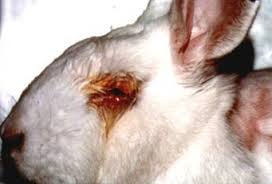
Here is a typical victim of the analysis we are going to learn today. Click on the image for more details about cruelty on research animals.
Binary data: MCMC and probit etc(Aug 25)
Warm up with a hypothetical data set
The hypothetical poison data set used in class.
dat = read.csv('probdat.csv',head=T)
names(dat)
propDeath = with(dat,Death/Size)
with(dat,plot(Dose,propDeath))
with(dat,plot(Dose,qnorm(propDeath)))
with(dat,lm(qnorm(propDeath)~Dose))
Ordinal explanatory variable: Snoring data
This data set is from our text book, and you may download it
snore.csv.
(dat = read.csv("snore.csv",head=T))
rowTot = apply(dat[,-1],1,sum)
prob = rowTot/sum(rowTot)

ridit=function(prob) {
  nCat = length(prob)
  sc=c(0,cumsum(prob)[-nCat])
  cat(sc)
  sc+prob/2
}

(x =  ridit(prob))

(propYes = dat[,2]/rowTot)
(probit = qnorm(propYes))
plot(x,probit)
(fit1 = lm(probit~x))

abline(fit1$coef)

(oddsYes = dat[,2]/dat[,3])
(logit = log(propYes))
plot(x,logit)
(fit2 = lm(logit~x))

abline(fit2$coef)
Horseshoe crab data set
The following photo taken from this web page shows a female horseshoe crab, its male mate and 4 satellite males.
 Here is the data set.
dat = read.table("crab.txt",head=T)
dim(dat)
head(dat)
tail(dat)
with(dat,plot(W,Sa))
with(dat,lines(lowess(W,Sa),col='red',lwd=3))
(fit = glm(Sa ~ W,family="poisson",data=dat))
summary(fit)

with(dat,plot(W,Sa,col=S))
with(dat,lines(lowess(W,Sa),col='red',lwd=3))
(fit = glm(Sa ~ W+as.factor(S),family="poisson",data=dat))
summary(fit)
CMH tests(Sep 22)
Our textbook discusses only the 2×2×k case. You may read about the generalised case from
the SAS documentation on generalised CMH test.
Multicategiry and ordinal logistic analysis (Oct 16)
allig = read.table('allig.txt',head=T)
#--------------------------------------
names(allig)
dim(allig)
#--------------------------------------
head(allig)
#--------------------------------------
library(nnet)
(fit = multinom(food ~ length, data=allig))
#--------------------------------------
pi.hat = fitted(fit)
pi.hat
#--------------------------------------
pi.hat %*% rep(1,3)
#--------------------------------------
plot(allig$length,pi.hat[,1],ylim=range(pi.hat),ty='l') #oops!
#--------------------------------------
ord = order(allig$length)
plot(allig$length[ord],pi.hat[ord,1],ylim=range(pi.hat),ty='l')
#--------------------------------------
lines(allig$length[ord],pi.hat[ord,2],col='red')
lines(allig$length[ord],pi.hat[ord,3],col='blue')
#--------------------------------------
allig$food
#--------------------------------------
relevel(allig$food,ref="O"))
#--------------------------------------
allig$food2 = relevel(allig$food,ref="O")
(fit2 = multinom(food2 ~ length, data=allig))
#---------Loading a data in dta format (used by STATA)
library(foreign)
#--------------------------
dat = read.dta("hsbdemo.dta")
#read.dta("http://www.ats.ucla.edu/stat/data/hsbdemo.dta")
#--------------------------
dim(dat)
names(dat)
head(dat)
#--------------------------
(fit = multinom(prog ~ ses + write, data = dat))
#--------------------------
summary(fit)
#--------------------------
names(summary(fit))
#--------------------------
(testStat = summary(fit)$coeff/summary(fit)$standard.errors)
#--------------------------
(1 - pnorm(abs(testStat))) * 2
#------------------------
frq = c(44,47,118,23,32,
18,28,86,39,48,
36,34,53,18,23,
12,18,62,45,51)

gender = c("F","M")

party = c("Dem","Rep")

ideology = 1:5
#--------------------------

dat = data.frame(expand.grid(ideology,party,gender),frq)

names(dat) = c("ideo","party","gender","frq")
#--------------------------

ftable(xtabs(frq~ideo+party+gender,dat))
#--------------------------
library(MASS)
fit = polr(ideo~party+gender,weight=frq,data=dat) #oops
#--------------------------
fit = polr(as.factor(ideo)~party+gender,weight=frq,data=dat)
(fit=polr(as.factor(ideo)~party,weight=frq,data=dat))
summary(fit)
#---------------------
confint(fit)
Structural Equation Modelling (Nov 03)
Today we shall fit a structural equation model (SEM) to a real life data collected by a wellknown
company in Kolkata. The data were collected by using a
questionnaire where most of the questions were to be answered in
a 7-point Likert scale.
We first load the relevant packages.
library(sem)
library(psych)
Now load the data set.
dat = read.table("data.txt",head=TRUE)
In this example we shall focus on only
the following items.
- 116(a): To what extent do policies and systems exist with respect to Work Organization ?
- 116(b): To what extent do policies and systems exist with respect to Performance Appraisal ?
- 116(c): To what extent do policies and systems exist with respect to Salary and Benefits ?
- 116(d): To what extent do policies and systems exist with respect to Competence Development ?
- 116(e): To what extent do policies and systems exist with respect to Career Management ?
- 116(f): To what extent do policies and systems exist with respect to Information Sharing ?
- 117: To what extent are HR Policies and Systems formalized in writing ?
- 118: To what extent is the employee population covered by HR Policies and Systems ?
- 119: To what extent do you understand how HRM Policies and Systems work ?
- 120: To what extent does the HRM Function enjoy credibility ?
- 121: To what extent is the HRM Function given importance and status ?
- 122(a): (Are you satisfied with the) Recruitment and Selection
- 122(b): (Are you satisfied with the) Induction
- 122(c): (Are you satisfied with the) Work Design
- 122(d): (Are you satisfied with the) Remuneration
- 122(e): (Are you satisfied with the) Recognition
- 122(f): (Are you satisfied with the) Training and Development
- 122(g): (Are you satisfied with the) Performance Management
- 122(h): (Are you satisfied with the) Employee Communication
- 123: To what extent are investments made in and resources provided to the HRM Function ?
- 124: To what extent do the HRM Policies & Systems enable you to align your goals, needs & aspirations with the organization's goals, needs and aspirations ?
- 125(a): Exhibit leadership for HRM
- 125(b): Define and communicate HRM vision for the future
- 125(c): Educate and influence senior management on HRM issues
- 125(d): Have adequate knowledge of HRM practices
- 125(e): Are knowledgeable about competitors' HRM practices
- 125(f): Focus on the quality of HRM deliverables
- 125(g): Have the ability to link business imperatives to HRM policies and practices
We start by extracting the relvant columns of the data.
start = (1:ncol(dat))[colnames(dat)=="q116_a"]
end = (1:ncol(dat))[colnames(dat)=="q125_g"]

used = start:end;
Our aim is to fit the following SEM where "distinctiveness",
"visibility", "understandability", "legitimacy" and "relevance"
are latent variables.
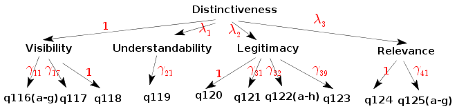 For each manifest variable we also have the double headed loop
arrows for variances that we have not shown in the diagram o
avoid clutter. The entire model in RAM notation is in the
file distmod.spc. The
extension
For each manifest variable we also have the double headed loop
arrows for variances that we have not shown in the diagram o
avoid clutter. The entire model in RAM notation is in the
file distmod.spc. The
extension .spc is just my arbitrary choice. Let us
take a look at a few lines from the file:
dist -> vis, NA, 1
dist -> und, lam1, NA
dist -> leg, lam2, NA
dist -> rel, lam3, NA
The general syntax for expressing a single-headed straight arrow
is like
from -> to , parameter name, initial value
If the parameter name is NA, then the arrow has a prespecified
value associated with it (the initial value). If the initial
value is NA, then R chooses its own suitable initial value. It is
possible to associate the same parameter with multiple
arrows. Just use the same parameter name, as done below.
vis -> q116_a, gam11, NA
vis -> q116_b, gam11, NA
The double-headed loop arrow syntax is similar:
dist <-> dist, sig0, NA

vis <-> vis, sig1, NA
und <-> und, sig1, NA
Next we have to load the model into R.
mod1 = specifyModel("distmod.spc")
SEM does not use the raw data. It works with the correlation
matrix. It is important that the correlation matrix is
nonnegative definite. In presence of missing values this is a
problem, because then there are two ways to compute a correlation
matrix:
- when computing the (i,j)-th entry, use all cases where both
of these variables are available. Then the correlation matrix is
not gurateeed to be nonnegative definite.
- first throw away all cases with at least a single missing
value for some variable. Then compute all the correlations based
on the remaining data. This will always produce a nonnegative
definite matrix.
We can proceed in a naive way by treating the ordinal category
numbers as the scores, as doen below.
corMat1 = cor(dat[,used],use="complete.obs")
But a better altrrnative is to respect the ordinal nature of the
data, and use polychoric correlation. Unfortunately, the
polychoric function of R does handle missing values nicely. So we
need to fiter them out manually as follows:
bad = apply(dat[,used],1,function(x) any(is.na(x)))
corMat2 = polychoric(dat[!bad,used])
Finally we can fit the SEM.
res = sem(mod1,corMat1,66) #oops!
res = sem(mod1,corMat1,66,maxiter=200)
If we want to use the polychoric correlation matrix then:
res = sem(mod1,corMat2$rho,66)